How to use 2D Fourier analysis to clean the noise in an image

Question

I have some other method to do this.But I desire to know how to use Fourier analysis to realize it.

---

I found a base post about Fourier-analysis to use in Image-Processing--Calculate the 2D Fourier transform of an Image.As the post

pic = ExampleData[{"TestImage", "Lena"}];
picdata = pic // ImageData;
picNoise = 
 ImageAdd[pic, 
  Image[RandomChoice[{.8, .2} -> {0, .3}, ImageDimensions[pic]]]]

Then we get its spectrum:

picFourier = 
 Fourier[picdata*
     PadRight[{{}}, 
      Most[picdata // Dimensions], {{1, -1}, {-1, 1}}]] // Abs // 
  Image

Let's do something in this spectrum,such as

dataProcess = CommonestFilter[picFourier, 1]

But how to reconstruct a image from spectrum we have precessed?Maybe it a very basic question,But I'm look forward your patient answer.

Answer 1

Here's what I did back in pre-MMA6 times. I believe you can easily adapt this method to work with all the fancy commands that have been added since then. Someone proficient in CDF programming could also make the mask building process interactive with disks and polygons: one window shows the FFT, the user places shapes to hide unwanted features, and another window shows the modified picture...

But let's go back in time: I started from a color image of a different kind of top model:

picture = Import["donald.bmp"];

This is a color bitmap, so it carries information about three colors per pixel. One should work on each color channel separately, and afterwards recombine the results into a single color picture. To make things brief, I'll work on a gray-scale version of the image. Back then I created one with this simple hack to convert to gray-scale (this procedure can create artifacts and there are better ways to convert to grayscale):

mat = picture[[1, 1]] /. {r_, g_, b_} :> (.3r + .6g + .1b)/1.;
{h, w} = Dimensions[mat]

{220,250}

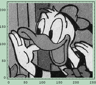
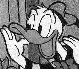
And here's my 'model'. Note the dithering in the image.

SetOptions[ListDensityPlot, Mesh -> False, AspectRatio -> Automatic];
orig = ListDensityPlot[mat]

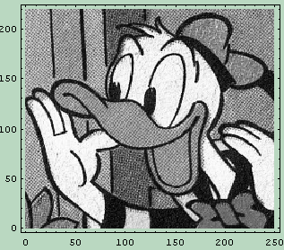
Admittedly, Lena looks better. Let's compute the FFT. We can do nice things with the amplitude alone (since ordinary photographs can encode only the amplitude of the light waves, we're not really losing anything).

fouriertransf = Fourier[mat];
Dimensions[fouriertransf]

{220,250}

This results in a shifted version of what you would 'see' in the focal plane of a lens

ListDensityPlot[Abs[fouriertransf]]

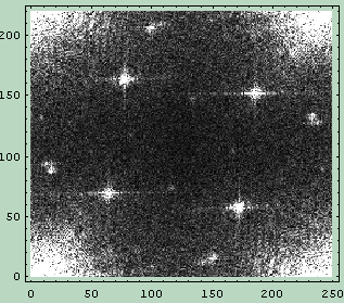
Now let's do some shifting. This is not strictly necessary, but I like to look at 2D FFTs as they 'appear' in the focal planes of a lens - it also helps in identifying low and high spatial frequencies; they are respectively at the center and at the border of the Fourier image.

hshift = IntegerPart[(h + .5)/2];
wshift = IntegerPart[(w + .5)/2];
fourierimage = Transpose[RotateLeft[
        Transpose[RotateLeft[
            fouriertransf,
            hshift]],
        wshift]];
ListDensityPlot[Abs[fourierimage]]

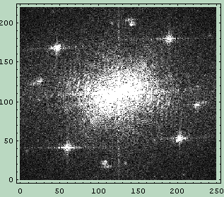
(some care is needed to discern between odd and even dimensions when doing the shifting. I did not exert such a care in my code, but today's built-in procedures will certainly take care of that for you. Just accept for the moment that some of my FFT might be slightly 'off-center').

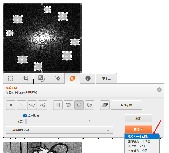
Ok, now we can create a mask that will act as a filter. Those 'star-like' features represent the FFT of the 'reticulate noise'. Let's try to get rid of them.

One very crude way to do it is by setting to zero the amplitude in their neighborhood. We can use step-like (or characteristic) functions to do that. In MMA this is easily and intuitively doable with Graphics directives.

The first thing we need are the coordinates of the 'star-like' spots; I extracted them from the FFT picture by hovering over them with the mouse while holding the CTRL key and by clicking to copy them.

bigpts = {{46, 170}, {188, 180}, {204, 53}, {61, 42}};
midpts = {{141, 201}, {223, 98}, {106, 25}, {22, 125}};
lilpts = {{9, 38}, {208, 7}, {226, 32}, {24, 193},
      {42, 216}, {241, 184}, {114, 16}, {136, 209}};

We now create disks of different sizes centered on those coordinates. Here's how our mask looks:

maskplot = Show[Graphics[{Disk[#, 11] & /@ bigpts,
         Disk[#, 8] & /@ midpts, Disk[#, 3] & /@ lilpts}, 
          PlotRange -> {{0, 250}, {0, 220}}, AspectRatio -> 
          Automatic, Background -> GrayLevel[1], ImageSize -> {250, 220}]];

Back then, I used this hack to convert it into a matrix of values

Export["mask.bmp", maskplot];
mask = Import["mask.bmp"][[1, 1]] /. {r_, g_, b_} :> (.3r + .6g + .1b)/1.;

Let's apply our mask to the FFT amplitude of our picture. By multiplying point by point, the amplitude is set to zero wherever there is a black pixel in the mask:

filteredfourier = fourierimage*mask;
ListDensityPlot[Abs[filteredfourier]];

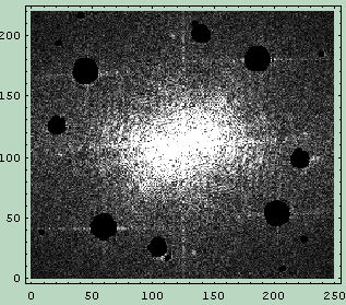
It's crude, I know. But it works:

filteredpic = InverseFourier[filteredfourier];
clean = ListDensityPlot[Abs[filteredpic]]

Side by side comparison with the original shows the reticulation is (mostly) gone and you can now appreciate the texture of the paper (it was an old comics book):

Show[GraphicsArray[{orig, clean}], ImageSize -> 600]

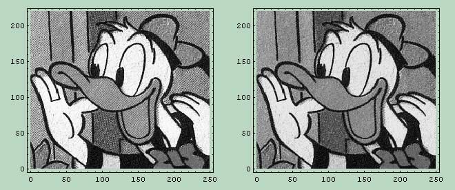
Also note how we did not lose details in the eyes and the lines of the hands.

Practically all of the proced--- hacks I've concocted have now direct, efficient (and most importantly correct) commands built-in in MMA. If you are using a post MMA6 version, you might also have to adapt the plotting function.

By the way, here's the (shifted) FFT of the mask:

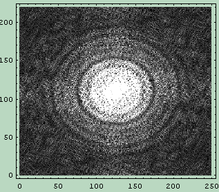
This is the 'point spread function (PSF)' that represents the noise we've removed. If you take an ideally clean picture where every single point of the image is a Dirac delta, and compute the convolution with a suitably scaled version of this PSF, you'll end up with an image with that sort of reticulation noise.

As pointed out in one of the comments, you can use graded filters instead of abrupt ones: by gradually transitioning from black (0) to white (1) you can create filters with the profiles that better suit your needs (Gaussian, Butterworth, Wiener, you name it...). The real magick (pun intended) happens when you can create an inverse filter, though, but that goes beyond this quick and dirty method. You can still do some pretty nice filtering, such as...

Low-pass noise filtering

Note: the procedures I am using from now on are just crude hacks to shorten the code. They will be defined at the end of this post.

Pseudo-periodic noise is not all of the story. Sometimes you might want to cut out the high frequency random noise by means of a low pass filter. You can create a rudimentary mask by using the negative of a disk centered in the spatial frequency origin. Take this picture for example (this is Karl Lambrecht, pioneer of calcite mining).

mat = GrayScaleMatrix["Karl.gif"];
dims = Dimensions[mat];
{hshift, wshift} = IntegerPart[(# + .5)/2] & /@ Dimensions[mat];
original = ListDensityPlot[mat, 
    MeshRange -> {{-wshift, wshift}, -hshift, hshift}}]

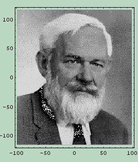
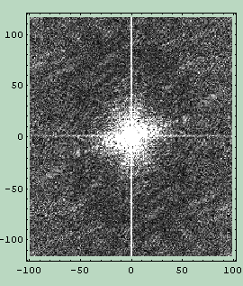
And here's its 2D FFT (still using the magnitude)

fft = FFT2D[mat];
ListDensityPlot[Abs[fft], MeshRange -> {{-wshift, wshift}, {-hshift, hshift}}]

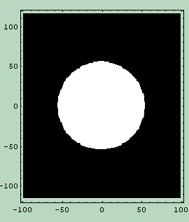
Our mask will be a low-pass filter created with a white disk on a black background. This is equivalent to a characteristic function that has value 1 inside the disk and goes abruptly to zero outside.

mask = MakeFilter[
      Graphics[{
          GrayLevel[0], Disk[{0, 0}, 160], GrayLevel[1], Disk[{0, 0}, 55]}
        ], dims, "mymask.bmp"];
ListDensityPlot[mask, MeshRange -> {{-wshift, wshift}, {-hshift, hshift}}]

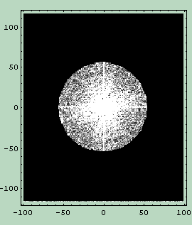
Again, we compute the product with the original FFT module (we apply our abrupt low-pass filter)

filtered = fft*mask;
ListDensityPlot[Abs[filtered], MeshRange -> {{-wshift,
   wshift}, {-hshift, hshift}}]

And then we go back to spatial coordinates. Rough, but somewhat effective (considering the clean-cut and incorrectly scaled mask):

filteredpic = InverseFourier[filtered];
clean = ListDensityPlot[Abs[filteredpic], MeshRange -> {{-wshift, wshift}, {-hshift, hshift}}]

Side by side comparison:

Show[GraphicsArray[{original, clean}], ImageSize -> 600]

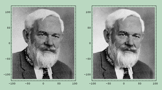
You might notice some 'ringing' especially localized at the borders of the image. A trick to remove that is to... not removing it but letting it happen to an additional average gray frame to be placed around your picture. If the frame is big enough, most of the ringing will take place in there. Your subsequently cropped filtered picture will be cleaner.

Structure filtering

And now, for something entirely different. Sometimes you can only go this far with a 'traditional' low-pass filter, but you may have knowledge of the underlying structure you are trying to dig out of the noise. This knowledge can help you create a spatial mask that will leave only the parts of the FFT that are compatible with such a structure. Let's see how far can you go with respect to a low-pass filter. First, we import the the image:

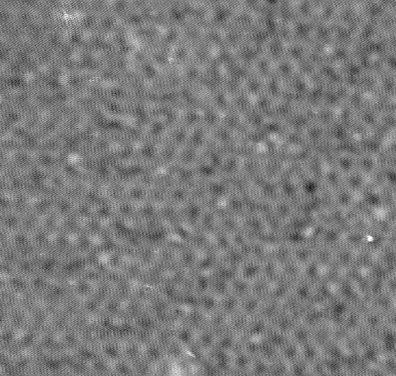
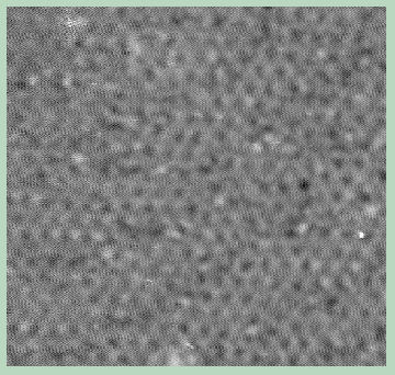
Not exactly and example of clarity and crispness. But we can see there's a periodic structure underneath all that noise. As usual we convert from color to grayscale and create a plot of the density matrix for comparing the results:

mat = GrayScaleMatrix["SEMscan.bmp"];
dims = Dimensions[mat];
{hshift, wshift} = IntegerPart[(# + .5)/2] & /@ Dimensions[mat];
original = ListDensityPlot[mat, Frame -> None]

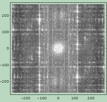
Here's the FFT (I am enhancing the FFT image by adding a logarithm; the original matrix is left untouched)

fft = FFT2D[mat];
ListDensityPlot[Log[10, Abs[fft]], MeshRange -> {{-
  wshift, wshift}, {-hshift, hshift}}]

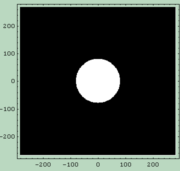
First thing we try is a low-pass filter. Old school. Here's the mask:

lowpassmask = MakeFilter[
      Graphics[{
          GrayLevel[0], Rectangle[{-wshift, -hshift}, {wshift, hshift}],
          GrayLevel[1], Disk[{1, 1}, 80]
          }
        ], dims, "mymask.bmp"];
ListDensityPlot[lowpassmask, MeshRange -> {{-
          wshift, wshift}, {-hshift, hshift}}]

And here's the filtered Fourier transform (enhanced via Log and with an added safety epsilon to avoid Log[0] errors from all that zero masking):

filtered = fft*lowpassmask;
ListDensityPlot[Log[10, Abs[filtered] + 0.01], MeshRange -> {{-wshift, \
wshift}, {-hshift, hshift}}]

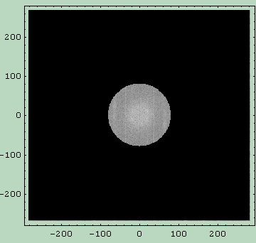
We gained a bit of clarity, but not that much.

filteredpic = InverseFourier[filtered];
lowpassClean = ListDensityPlot[Abs[filteredpic], Frame -> None]

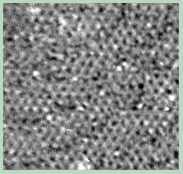
Sure, we could try to identify the source of the remaining noise and shape a new mask in a more fancy way, but there's a better way to highlight the structure we know to be there: we can throw everything away but what we want to see. Time for a new, smarter, mask:

lilpts = {{-17.9878, 12.0672}, {1.2213, 23.7626}, {18.797, 
      14.5501}, {18.797, -7.99123}, {2.07068, -17.2037}, {-14.6556, \
-12.1728}};

structuremask = MakeFilter[
      Graphics[{
          GrayLevel[0], Rectangle[{-wshift, -hshift}, {wshift, hshift}],
          GrayLevel[1], Disk[{1, 1}, 6],
          GrayLevel[1], Disk[#, 6] & /@ lilpts
          }
        ], dims, "mymask.bmp"];
ListDensityPlot[structuremask, MeshRange -> {{-wshift, wshift}, {-hshift, 
          hshift}}]

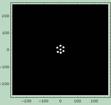
Note that I had to use {1,1} for the origin. This is due my the poorly implemented shifting of the FFT. As I probably already said six or seven times already, I was in a hurry to see pretty pictures. Exactness was not one of my goals. The filtered FFT is deceptively insignificant:

filtered = fft*structuremask;
ListDensityPlot[Log[10, Abs[filtered] + 0.01], MeshRange -> {{-
  wshift, wshift}, {-hshift, hshift}}]

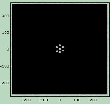
But it carries all the information we want to see:

filteredpic = InverseFourier[filtered];
structureClean = ListDensityPlot[Abs[filteredpic], Frame -> None]

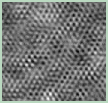
Better? Yep, it's graphene. Wasn't it clear from the start?

As usual, here's a side by side comparison: original, low-pass filtered and structure-filtered:

Show[GraphicsArray[{original, lowpassClean, structureClean}], ImageSize -> 600];

Caveat emptor: what we see in the last picture here, is what we wanted to see; in a way it is as if the image had been warped to suit the hexagonal structure we suppose is there.

Final considerations

The examples I've made here are the simplest possible imaginable. Yet, they can be very effective, even with such crude, rudimentary and ill-shaped masks (and FFT shifting procedure). In general, random noise can be filtered by some sort of low-pass mask, and you can probably get better results by adopting a gradual transition from 1 to 0 (for example with a gaussian or sigmoidal profile).

The filtering method is completely general and not limited to this graphical approach. The FFT of the mask is the point spread function that can be used to create the noisy image by means of a convolution with the clean image.

Basically, what is needed is the (numerical) deconvolution of the noisy image and the point spread function that represent the effect of the added noise on a Dirac delta in the origin (some might call that the impulse response of the system). When you have identified the PSF, you 'just' divide the FFT of the noisy image by the FFT of the PSF (it can get tricky when you have to avoid division by zero, but that's the general idea). By going mathematical, things can get really fancy: you can identify the point spread function in a blurred picture (due to movement in the camera or in the subject) and de-blur it very effectively. Here you can see an example of that kind.

Yet, this primitive graphical method is very intuitive and in my opinion also educative.

One can find introductory chapters to optical Fourier filtering on most mainstream optics textbook such as Pedrotti & Pedrotti, Guenther, and Hecht. To go further, I suggest the following books:

Fourier Optics An Introduction, 2nd edition E. G. Steward, Dover (Brief, inexpensive and with some cool examples)

Introduction to Fourier Optics, 3rd edition J. W. Goodman, Roberts & Company (The bible, but not exactly for beginners and most importantly not focused on image processing)

Procedures (nothing fancy, just to shorten the code)

Please note, these are just crude hacks I put together back then to get to the pictures in the least possible time. They are incorrect: the gray scale converter creates artifact, and the FFT2D procedure has problem with odd dimensions. MakeFilter leaves garbage masks in your current directory. They are here just because I used them back then, and they help in reducing the code above.

GrayScaleMatrix[filename_String] := Module[{pic},
    pic = Import[filename];
    pic[[1, 1]] /. {r_, g_, b_} :> (.3r + .6g + .1b)
    ]

FFT2D[mat_] := Module[{ft, hshift, wshift},
    ft = Fourier[mat];
    {hshift, wshift} = IntegerPart[(# + .5)/2] & /@ Dimensions[ft];
    Transpose[RotateLeft[
        Transpose[RotateLeft[
            ft,
            hshift]],
        wshift]]
    ]

MakeFilter[obj_, {h_, w_}, filename_String:"tempfilt.bmp"]:=
 Block[{$DisplayFunction = Identity, hs, ws, pic},
    {hs, ws} = IntegerPart[(# + .5)/2] & /@ {h, w};
    pic = Show[obj, PlotRange -> {{-ws, ws}, {-hs, hs}}, 
    ImageSize -> {w, h}, 
        AspectRatio -> Automatic, Frame -> False, Background -> GrayLevel[1]];

    Export[filename, pic];
    GrayScaleMatrix[filename]
    ]

Answer 2

Make the answer of Peltio to be readable in following:

grayImg = 
 Uncompress[
  FromCharacterCode[
   Flatten[ImageData[Import["https://i.sstatic.net/SzwMi.png"], 
     "Byte"]]]]

fourierimage = ResourceFunction["FourierShift"][Fourier[ImageData[grayImg]]];
Image[Abs[fourierimage]]

Get the mask by the image tool:

Import["http://halirutan.github.io/Mathematica-SE-Tools/decode.m"]["https://i.sstatic.net/PLmnx.png"]
Image[Abs[InverseFourier[ResourceFunction["FourierShiftInverse"][fourierimage*ImageData[ColorNegate[mask]]]]]]