The problem is more involved than I thought.
This post involves several code blocks, you can copy them easily with the help of importCode.
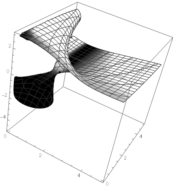
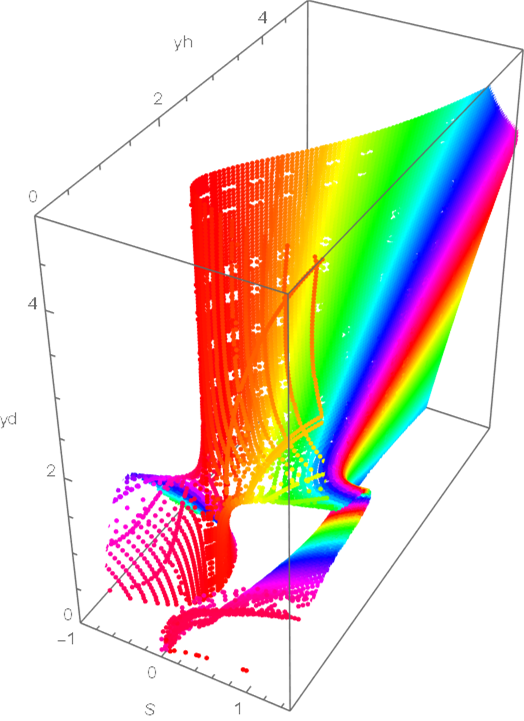
Based on Ulrich Neumann's idea i.e. transforming the $(x_h, y_h, y_d)$ coordinates to $(S,y_h,y_d)$ coordinates, we transform the contour surface directly as follows:
M = 1;
roo = 0.01;
xd = 3;
sys = {(2 M (xh^2 - (yh + 1)^2))/(xh^2 + (yh + 1)^2)^2 + (
        2 S ((xh - xd)^2 - (yh + yd)^2))/((xh - xd)^2 + (yh + yd)^2)^2 + J/(2 yh) == 0,
       (M xh (yh + 1))/(xh^2 + (yh + 1)^2)^2 + (
        S (xh - xd) (yh + yd))/((xh - xd)^2 + (yh + yd)^2)^2 == 0,
       J Log[(2 yh J)/roo] + (2 M (yh + 1))/(xh^2 + (yh + 1)^2) + (
        2 S (yh + yd))/((xh - xd)^2 + (yh + yd)^2) == Log[2/roo] + 1};

ruleJS = Solve[sys // Most, {J, S}] // Flatten;

eqmid = sys[[3]] /. ruleJS;

Sfunc[xh_, yh_, yd_] = S /. ruleJS;

plot = ContourPlot3D[
      0 == Subtract @@ eqmid // Evaluate,
      {xh, -5/2, 7/2}, {yh, 0, 4}, {yd, 0, 6},
       PlotPoints -> 20]; // AbsoluteTiming
(* {208.254, …} *)

Show[plot /.
    GraphicsComplex[lst_, rest__] :>
      GraphicsComplex[
        Function[{xh, yh, yd}, {Sfunc[xh, yh, yd], yh, yd}] @@
            Transpose@lst // Transpose, rest],
  AxesLabel -> {S, Subscript[y, h], Subscript[y, d]},
 ViewPoint -> {1.2, 0.7, -3.}, ViewVertical -> {-1, 1, 1},
 BoxRatios -> Automatic,
 PlotRange -> {{-1, 3/2}, {0, 4}, {0, 6}}]
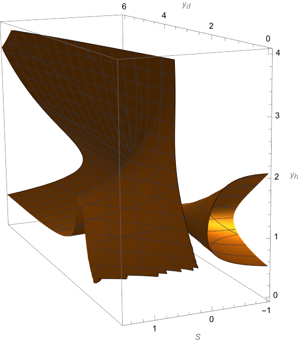
Remark
The equation has been defined in a strange manner i.e. 0 == Subtract @@ eqmid to circumvent the following bug:
ContourPlot3D wrong plotting result with extra surfaces
Do notice this work-around is not robust. Personally I recommend
turning back to a earlier version like v8 or v9 to circumvent the
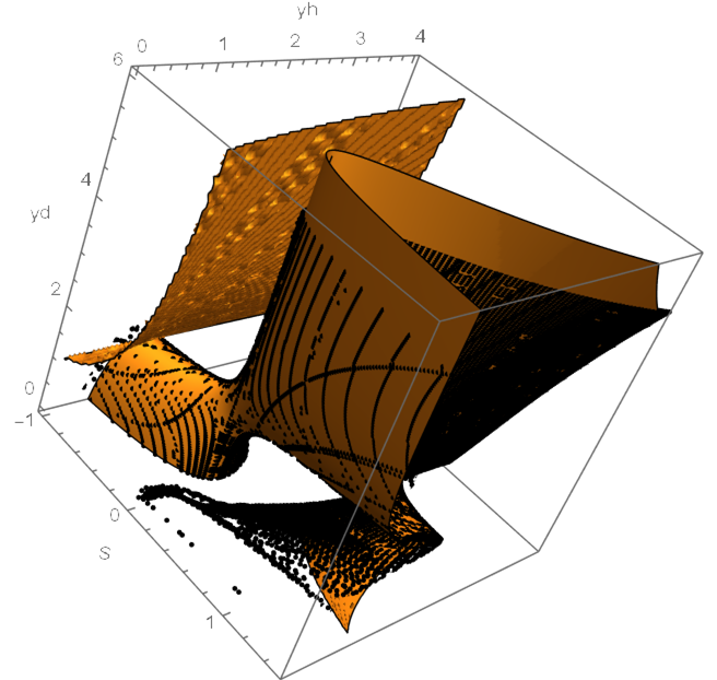
bug. The following is the output in v8:
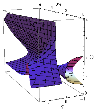
As we can see, the surface is plotted better.
If you just want to know how to plot the surface, you can stop here.
Further Analysis
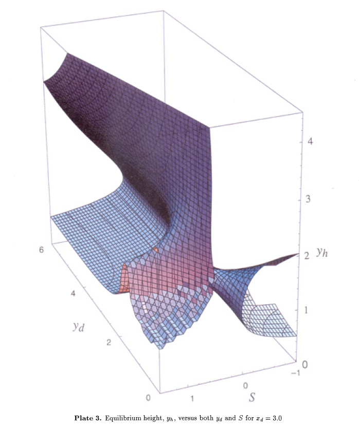
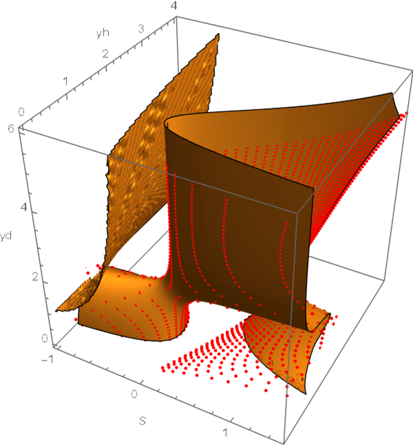
If you carefully compare the plot in the paper to ours, you may notice that, the surface in the region yd < 3 && yh < 2 && s > 0.5 seems to be slightly inconsistent (even if we ignore the roughness of the result in paper). I suspect the surface in the paper hasn't been plotted in a correct way.
The following is a way to produce a contour surface that's closer to that in paper. The idea itself is simple: we directly eliminate the redundant J and xh, and plot the remaining equation. J is easy to eliminate, because the first equation is a linear equation of J, so it can be Solved easily:
rule1 = Solve[sys[[1]], J] // Flatten
The troublesome part is xh. We can obtain a 5th order polynomial equation of xh by taking numerator of sys[[2]], but as mentioned in the question, xh∈Reals, so only one of the real root is needed. Which real root should be chosen? Additionally, how can this be done in an efficient way?
To speed up the code, I'll turn to the function roots in this post:
roots[c_List] := Block[{a}, a = DiagonalMatrix[ConstantArray[1., Length@c - 2], -1];
   a[[1]] = -Rest@c/First@c;
   Eigenvalues[a]];
I haven't used the more efficient method based on librarylink mentioned therein because I'm too lazy I don't want to make this answer too advanced.
With roots, we build the following function for solving xh:
takenume = (Subtract@@#//Together//Numerator)&;
(xhfunc[S_, yh_, yd_?NumericQ] := First@Sort@Cases[Chop@roots[#], _Real]) &@
 Reverse@CoefficientList[takenume@sys[[2]], xh]
Here I've simply chosen the smallest Real root of the equation. This is merely a guess. But later we'll see this guess indeed reproduces the picture in paper.
By substituting J and xh to last equation, we obtain an equation that can be plotted by ContourPlot3D. To improve the efficiency, we Compile the obtained equation:
lhs3compiled =
  Compile[{S, yh, yd, xh},
   sys[[3]] /. rule1 // Subtract@@#& // Evaluate,
   RuntimeOptions -> EvaluateSymbolically -> False];
And we write the following code for visualization:
(* The minus sign is for circumventing the aforementioned bug. *)
ContourPlot3D[
  -lhs3compiled[S, yh, yd, xhfunc[S, yh, yd]],
  {S, -1, 3/2}, {yh, 0, 4}, {yd, 0, 6}, Contours -> {0},
  AxesLabel -> Automatic, BoxRatios -> Automatic,
  ViewPoint -> {1.2, 0.7, -3.}, ViewVertical -> {-1, 1, 1}] // AbsoluteTiming
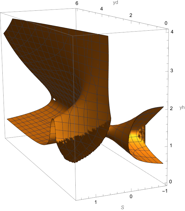
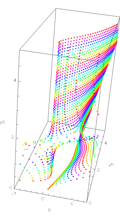
As we can see, the surface in the region yd < 3 && yh < 2 && s > 0.5 is closer to the one in the paper, but this is probably the result of numeric error. Let's take a slice and observe at S = 3/2:
With[{S = 3/2}, Plot3D[
      lhs3compiled[S, yh, yd, xhfunc[S, yh, yd]], {yd, 0, 6}, {yh, 0, 4},
  AxesLabel -> Automatic, PlotRange -> All,
  ScalingFunctions -> {"Reverse", Automatic}, Mesh -> {{0}}, MeshFunctions -> {#3 &},
   PlotPoints -> 50]]
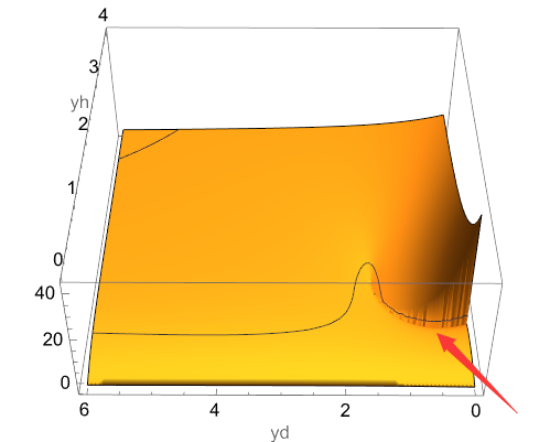
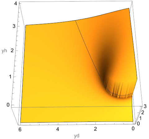
As shown above, there's a sudden jump at the region yd < 3 && yh < 2, and the zero contour actually lies on the cliff wall. Further check suggests the cliff is generated by xhfunc, which involves the artificial "take the smallest real root" operation that's likely to generate jump in solution:
With[{S = 3/2}, Plot3D[
      xhfunc[S, yh, yd], {yd, 0, 6}, {yh, 0, 4}, AxesLabel -> Automatic,
  PlotRange -> All, ScalingFunctions -> {"Reverse", Automatic}, Mesh -> {{1}},
  MeshFunctions -> {#3 &}, PlotPoints -> 50]]
With[{S = 3/2}, ContourPlot[
    {0 == lhs3compiled[S, yh, yd, xhfunc[S, yh, yd]],
   xhfunc[S, yh, yd] == 1}, {yd, 0, 6}, {yh, 0, 4}, FrameLabel -> Automatic,
  PlotPoints -> 50, ScalingFunctions -> {"Reverse", Automatic}]]
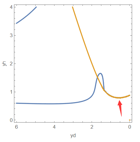
Of course, the illustration above is inadequate to prove the new surface is fake, but I think it's at least plausible.



{f1, f2, f3}in terms of{x, y, x, a, b}. $\endgroup$xh? $\endgroup$