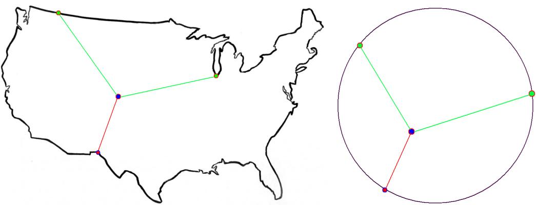
If the domain $\varOmega$ of the county is simply connect, one might use the Riemannian mapping theorem.
For $z_0 \in \varOmega^\circ$, we make the following ansatz for the holomorphic map $f \colon \varOmega \to D^2$:
$$ f(z) = (z-z_0) \, \operatorname{e}^{u(z) + \operatorname{i}\!v(z)}.$$
Then $|f(z)| = |z-z_0| \, \operatorname{e}^{u(z)}$ has to equal $1$ for all $z \in \partial \varOmega$. The Cauchy-Riemann equations imply that $u$ is the unique solution to the following Poisson problem:
$$\begin{cases}
\Delta u(z) &= 0, &z \in \varOmega^\circ,\\
u(z) &= - \log( |z-z_0|), &z \in \partial \varOmega.
\end{cases}$$
#Implementation of $u$
This can be easily solved with the finite element method. Here is how this can be done (I chose a different country because the boundary curve of the USA seemed to have self-intersections):
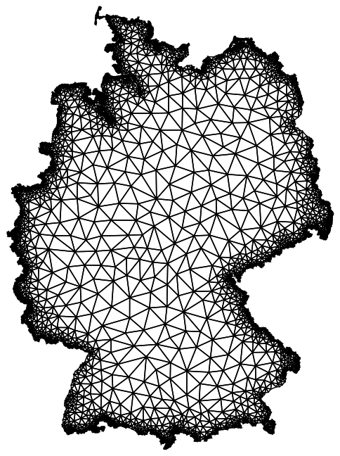
First, we discretize the interior of the domain:
Needs["NDSolve`FEM`"];
p = Most@Cases[CountryData["Germany", "Shape"], _Polygon, \[Infinity]][[1, 1, 1]];
R = ToElementMesh[
   BoundaryMeshRegion[p, Line[Partition[Range[Length[p]], 2, 1, 1]]],
   "MeshOrder" -> 1,
   MaxCellMeasure -> {1 -> .01}
   ];
R["Wireframe"]

(*Initialization of Finite Element Method*)

vd = NDSolve`VariableData[{"DependentVariables", "Space"} -> {{u}, {x, y}}];
sd = NDSolve`SolutionData[{"Space"} -> {R}];
cdata = InitializePDECoefficients[vd, sd,
   "DiffusionCoefficients" -> {{-IdentityMatrix[2]}},
   "MassCoefficients" -> {{1}}
   ];
bcdata = InitializeBoundaryConditions[vd, sd, {DirichletCondition[u[x, y] == 0., True]}];
mdata = InitializePDEMethodData[vd, sd];

(*Discretization*)
dpde = DiscretizePDE[cdata, mdata, sd];
dbc = DiscretizeBoundaryConditions[bcdata, mdata, sd];
{load, stiffness, damping, mass} = dpde["All"];
DeployBoundaryConditions[{load, stiffness}, dbc];

(*Preparation of Dirichlet boundary conditions for u*)

bndedges = R["BoundaryElements"][[1, 1]];
bndvertices = Sort@DeleteDuplicates[Flatten[bndedges]];
bpts = R["Coordinates"][[bndvertices]];
z0 = {0., 0.};
b = ConstantArray[0., Length[R["Coordinates"]]];
b[[bndvertices]] = -0.5 Log[Total[(bpts - ConstantArray[z0, Length[bpts]])^2, {2}]];

(*Solving the system and creating an interpolating function*)

solver = LinearSolve[stiffness, Method -> "Pardiso"];
uvals = solver[b];
ufun = ElementMeshInterpolation[{R}, uvals];
#Implementation of $v$
Due to the Cauchy-Riemann equations, we have
$$\operatorname{grad}(v) = J \, \operatorname{grad}(u),$$
where $J$ is the rotation of 90 degrees in counter clockwise orientation. Since $\varOmega$ is simply connected, up to a constant, $v$ is defined uniquely by this relation.
Hence, $v$ is also harmonic and is a solution of the following Neumann problem:
$$\begin{cases}
\Delta v(z) &= 0, &z \in \varOmega^\circ,\\
\frac{\partial v}{\partial \nu} (z) &= \langle \nu(z) , J \operatorname{grad}(u)(z) \rangle, &z \in \partial \varOmega.
\end{cases}$$
This pde is also amenable to a treatment with finite elements, although the preparation of the Neumann data needs a bit of fiddling. Notice that this second equation determines $v$ only up to a constant shift, which corresponds to the fact that $f$ is also unique up to a rotation of the disk.
(*Preparation of Neumann boundary conditions for v*)

gradu = {x, y} \[Function] Evaluate[D[ufun[x, y], {{x, y}, 1}]];
J = N@RotationMatrix[Pi/2];
p = R["Coordinates"];
{i, j} = Transpose[R["BoundaryElements"][[1, 1]]];
normalprojections = MapThreadDot[R["BoundaryNormals"][[1]], (gradu @@@ (0.5 (p[[i]] + p[[j]]))).(-J)];
boundaryedgelengths = Sqrt[Total[(p[[i]] - p[[j]])^2, {2}]];
{α, β} = Transpose[bndedges];
vertexbndedgeconnectivity = SparseArray[
   Transpose[{
      Join[α, β],
      Join[Range[Length[α]], Range[Length[β]]]
      }] -> 1,
   {Length[p], Length[bndedges]}
   ];

(*Solving the system and creating an interpolating function*)

b = vertexbndedgeconnectivity.(normalprojections boundaryedgelengths);
vvals = solver[b];
vfun = ElementMeshInterpolation[{R}, vvals];
Finally, we can obtain our approximation to the Riemannian mapping $f \colon \varOmega \to D^2$ by
f = {x, y} \[Function] Evaluate[
    ComplexExpand[
     ReIm[((x + I y) - (z0[[1]] + I z0[[2]])) Exp[ufun[x, y]] (Cos[vfun[x, y]] + I  Sin[vfun[x, y]])]
     ]
    ];
#Visualization
First, my favorite texture.

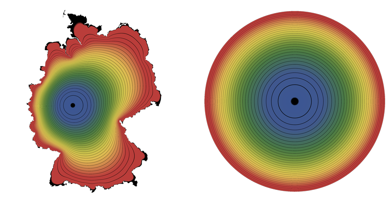
Now, the actual plots, using basically $f$ as texture map for $\varOmega$. (Plots were obtained with resolution MaxCellMeasure -> {1 -> .001}.)
tex = Import["https://i.sstatic.net/gRwc1.png"];
texcoords = Transpose[{
    Total[(f @@@ p)^2, {2}],
    ConstantArray[0.5, Length[p]]
    }];
g = GraphicsRow[{
   Graphics[{Texture[tex],
     ElementMeshToGraphicsComplex[R, VertexTextureCoordinates -> texcoords]
     }],
   Graphics[{Texture[tex],
     ElementMeshToGraphicsComplex[R, VertexTextureCoordinates -> texcoords,
      "CoordinateConversion" -> (f @@@ # &)]
     }]
   },
  ImageSize -> Full
  ]
