How to find max difference with the same x between two functions?

Question

For example, I have function

TF[y_] = 2 / Pi * ArcSin[y]

And I have CDF:

SeedRandom[10]
sample = Sort[Sin[pi*RandomVariate[UniformDistribution[{0, 1}], n]]];
D = EmpiricalDistribution[sample];
EF = CDF[D, x], where is x = {0, 1}

How to find max difference between functions values with the same x? Is it possible to build same plot?

Answer 1

ClearAll[tF]
SeedRandom[10]
n = 100;
sample = Sort[Sin[Pi*RandomVariate[UniformDistribution[{0, 1}], n]]];
dist = EmpiricalDistribution[sample];

Use tF to define a custom ProbabilityDistribution:

tF[y_] := 2/Pi*ArcSin[y]
tfdist = ProbabilityDistribution[{"CDF", tF[x]}, {x, 0, 1}];
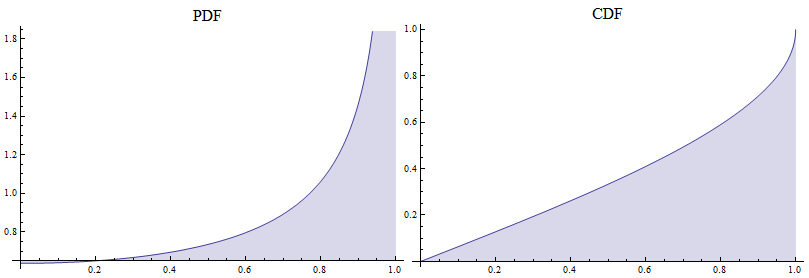
Row[Plot[Evaluate[#[tfdist, x]], {x, 0, 1}, Filling -> Axis, 
    ImageSize -> 400, PlotLabel -> Style[#, 16]] & /@ {PDF, CDF}]

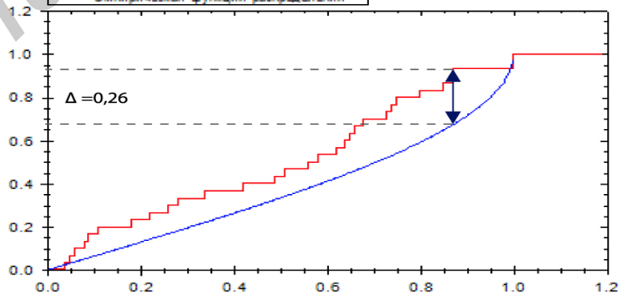
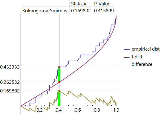
KolmogorovSmirnovTest is based on the maximum difference between CDFs of two distributions.

ksts = KolmogorovSmirnovTest[sample, tfdist, "TestStatistic"]

0.169802

f1 = CDF[dist, #] &;
f2 = CDF[tfdist, #] &;
MaxValue[{Abs[f1[x] - f2[x]], -1 < x < 1}, {x}]

0.169802

xv = ArgMax[{Abs[f1[x] - f2[x]], 0 < x < 1}, {x}][[1]];
yv = Through@{f1[#] - f2[#] &, f1, f2}@xv;
points = Thread[{xv, yv}];
tsttable = Style[#, "Panel", 16]&@@ KolmogorovSmirnovTest[sample, tfdist, "TestDataTable"];
legends = (Style[#, "Panel", 16] & /@ {"empirical dist", "tfdist", "difference"});

Plot[{f1[x], f2[x], f1[x] - f2[x]}, {x, 0, 1}, Exclusions -> None, 
 PlotRange -> All, PlotStyle -> Thick, PlotLegends -> legends, AspectRatio->1,
 ImageSize -> 500, LabelStyle -> {"Panel", 16}, PlotLabel -> tsttable,
 GridLines -> ({{xv}, yv}), Ticks -> {Automatic, yv}, 
 Prolog -> {Thickness[.025], Opacity[.9], Green, CapForm["Butt"],
  Line[Rest@points], Line[{First@points, {xv, 0}}], PointSize[Large], Red, Point[points]}]

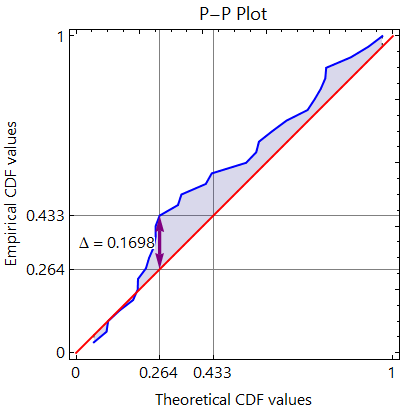
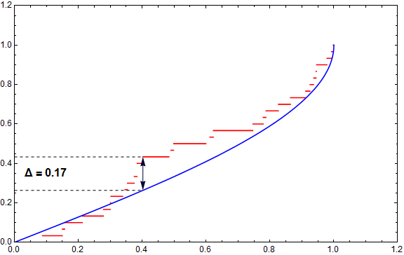
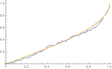
ProbabilityPlot: Empirical CDF values versus theoretical CDF values:

ProbabilityPlot[sample, tfdist, Joined -> True, 
 ReferenceLineStyle -> Directive[Thick, Dashing[None], Red], 
 PlotStyle -> Directive[Thick, Blue], ImageSize -> 400, LabelStyle -> {"Panel", 16},
 FrameTicks -> {Join[{0}, Round[yv[[{2, 3}]], .001], {1}], 
   Join[{0}, Round[yv[[{2, 3}]], .001], {1}], Automatic, Automatic}, 
 AspectRatio -> 1, GridLines -> ({yv[[{2, 3}]], yv[[{2, 3}]]}),
 Filling -> {1 -> {2}}, PlotLabel -> Style["P-P Plot", 18],
 FrameLabel -> { "Theoretical CDF values", "Empirical CDF values"}, 
 Epilog -> {Text[Style["\[CapitalDelta] = " <> 
      ToString[Round[Subtract @@ yv[[{2, 3}]], .0001]], 16, "Panel"], 
      {yv[[3]]/2, Mean@yv[[{3, 2}]]}],
   Purple, Arrowheads[{-.05, .05}] , Thickness[.01], 
   Arrow@ Line[{yv[[{3, 2}]], yv[[{3, 3}]]}]}]

See also: What is the formula behind the Kolmogorov-Smirnov test statistics?

Answer 2

Also fixing your code...

n=30;
TF[y_] = 2/Pi*ArcSin[y];
SeedRandom[10];
sample = Sort[Sin[Pi*RandomVariate[UniformDistribution[{0, 1}], n]]];
d = EmpiricalDistribution[sample];
EF = CDF[d, x];

To get the max. difference, I tried NMaximize and others, but didn't work. The one that worked for me was this:

X = NArgMax[{Abs[EF - TF[x]], 0 < x < 1}, x]
maxDIF = Abs[EF - TF[x]] /. x -> X
(*0.402233*)
(*0.169802*)

Plot:

Show[
 Plot[{EF, TF[x]}, {x, 0, 1}, PlotRange -> {{0, 1.2}, {0, 1.2}},
  PlotStyle -> {Red, Blue},
  Frame -> True, FrameStyle -> Directive[Black, 12], ImageSize -> Large],

 Graphics[{Darker[Blue, 0.8], Arrowheads[{-.025, .025}], 
          Arrow[{{X, TF[X]}, {X, EF /. x -> X}}]}],
 Graphics[{Dashed, Line[{{0, TF[X]}, {X, TF[X]}}]}],
 Graphics[{Dashed, Line[{{0, EF /. x -> X}, {X, EF /. x -> X}}]}],
 Graphics[
          Text[ 
             "\[CapitalDelta] = " <> ToString[Round[maxDIF, 0.01]],
             { 0.1,Mean[{TF[X], EF /. x -> X}] },
             BaseStyle -> {Bold, FontSize -> 16}
              ]]
 ]

Answer 3

You had a few oddities in your syntax.

• If you want to define TF as a function of $y$, you had best use SetDelayed (:=) instead of set. Take a look at the documentation of search this site on this point.
• The constant $\pi$ is Pi in Mathematica, note the uppercase letter.
• $n$ was not defined in your code. I am arbitrarily using $100$ data points in the expression below. Adjust as needed.
• D is reserved for the derivative function. More in general, you should avoid all uppercase variable names, especially the single-letter ones, as they may conflict with built-in symbols.

---

Take a look at the code below, I think it might be close to what you want:

Clear[TF, EF, sample, dist]

TF[y_] := 2/Pi*ArcSin[y]

SeedRandom[10]
sample = Sort[Sin[Pi*RandomVariate[UniformDistribution[{0, 1}], 100]]];
dist = EmpiricalDistribution[sample];
EF[y_] := CDF[dist, y]

Plot[{EF[y], TF[y]}, {y, 0, 1}]

Then the difference is simply:

Plot[EF[y] - TF[y], {y, 0, 1}]