Changing the data indices for a large dataset plotted with ContourPlot

Question

I have a large (square) dataset that I am plotting with ListContourPlot ... The data is 128x128 -- without coordinates for each point. I.e. -

{{0,0,1,0,...,0},{0,2,1,1,...,1},...{3,1,1,1,...,2}}

So the default contour plot uses the axis range 0->128 - for both x and y since there are 128 sets of 128 points.

However, how can I remap the axis such that I plot this data with axis ranges of {-150,150}?? I realize that Rescale will give the formula to remap 128 points to the range -150,150 (e.g. - X/128 * 300 - 150), but how do I tell ListContourPlot to use those indices for the data (and hence those tick marks)?

Thx,

Rick

Answer 1

per my comment, without DataRange

ListContourPlot[Table[Sin[i + j^2], {i, 0, 3, 3/128}, {j, 0, 3, 3/128}]]

...and with

ListContourPlot[Table[Sin[i + j^2], {i, 0, 3, 3/128}, {j, 0, 3, 3/128}], 
   DataRange -> {{-150, 150}, {-150, 150}}]

Answer 2

I interpret the question as rescaling. I accept that the OP wished to avoid Rescale, however, I post this a way to achieve what I understand is the goal. Note, that this could be simplified for square data and as interpolation will have with more than small scale changes.

func[dt_, xl_, xu_, yl_, yu_] := Module[{dim, res1, res2,t},
  dim = Dimensions[dt];
  res1 = Rescale[t, {1, dim[[1]]}, {yl, yu}];
  res2 = Rescale[t, {1, dim[[2]]}, {xl, xu}];
  Flatten[
   MapIndexed[{Sequence @@ {res2 /. t -> #2[[2]], 
        res1 /. t -> #2[[1]]}, #1} &, dt, {2}], 1]
  ]

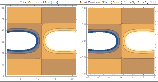
An example:

tb = Table[
   Cos[i] Sin[j] Exp[-(i^2 + j^2)], {i, -3, 3, 0.1}, {j, -1, 1, 0.1}];
lc = ListContourPlot[tb, ImageSize -> 300];
lcf = ListContourPlot[func[tb, -3, 3, -1, 1], ImageSize -> 300];
Grid[{{HoldForm[ListContourPlot[tb]], 
   HoldForm[ListContourPlot[func[tb, -3, 3, -1, 1]]]}, {lc, lcf}}, 
 Frame -> All]