9
$\begingroup$

I'm trying to numerically integrate a function which has a vector-valued slow part and a much faster component which is shared by all the components, i.e. an integral of the form $$ \int_a^b\begin{pmatrix}f(x)\\ g(x) \\ h(x)\end{pmatrix}w(x)\,\text dx. $$ Because NIntegrate is nicely Listable on its first argument, I can feed it a list-valued argument without a problem. However, it appears to be doing each component as a completely separate integral, which results in a lot of work being re-calculated.

For example, the (simplified) example integral

samplePointsList = Reap[
    NIntegrate[
     {x, x^2, x^3} Cos[10 x + Cos[x]]
     , {x, 0, 5}
     , EvaluationMonitor :> Sow[x]
     ]
    ][[2, 1]];

gives the sample point diagram (through ListPlot[Transpose[{samplePointsList, Range[Length[samplePointsList]]}]])
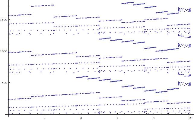
enter image description here

It is clear that the kernel is doing the initial sampling, and then the further refinements, separately for each component. While the required sample points are not identical, there is a lot of shared work and I feel there is a fair bit of room for optimization there.

I am aware that, since the sampling requirements of each component are slightly different, binding them completely will require more evaluations in some components than would be necessary. (For instance, in the example above, the extra detail required by the first component around $2\leq x\leq 3$ would be slowed down slightly if it was required to also calculate the second and third components there, though they do not require it.) However, the components in my case are similar enough that I do not think this would be an issue.

Is there a way to force Mathematica into this sort of separation of the integrand and unification of the sampling? If not, is there a way to make it aware of the previously calculated values and sampling points which will speed up the process?

$\endgroup$

2 Answers 2

5
$\begingroup$

One idea is to integrate once to get the sample points then compute the remaining integrals as sums:

 sample = Transpose@
    SortBy[First@Last@Reap[
       NIntegrate[x (c = Cos[10 x + Cos[x]]), {x, 0, 5}, 
                  EvaluationMonitor :> Sow[{x, c}]]], #[[1]] &];
 wt = ((#[[3]] - #[[1]])/2) & /@ Partition[Join[{0}, sample[[1]], {5}], 3, 1];
 wt.(sample[[2]] #) & /@ {sample[[1]], sample[[1]]^2, sample[[1]]^3}

{0.0133333, 0.133275, 0.861541}

Note the accuracy is not terribly good, NIntegrate gives:

{0.0125266, 0.131514, 0.855716}

Somethings a bit off in my quick&dirty trapezoid integration but i think this can be made to work.

roll your own

For this example there really is little benefit to NIntegrate's adaptive sampling so we might as well just use a uniform sampling:

 np = 651;(*assumed odd for simpsons rule*)
 a=5
 b=0
 wt = ( (a-b)/(np - 1) )/3 Join[{1}, Flatten@ConstantArray[{4, 2}, (np - 1)/2 - 1], {4, 1}] // N;
 x = b + (Range[0, np - 1] (a-b)/(np - 1)) // N;
 fast = Cos[10 # + Cos[#]] & /@ x // N;
 (# fast).wt & /@ {x, x^2, x^3}

{0.0125266, 0.131514, 0.855716}

$\endgroup$
5
$\begingroup$

The answers to

Is there a way to force Mathematica into this sort of separation of the integrand and unification of the sampling? If not, is there a way to make it aware of the previously calculated values and sampling points which will speed up the process?

are "yes" and "yes" as demonstrated and discussed in this post to "How to calculate the numerical integral more efficiently?".

More concretely:

Import["https://raw.githubusercontent.com/antononcube/\
MathematicaForPrediction/master/Misc/ArrayOfFunctionsRule.m"]

funcExpr = {x, x^2, x^3} Cos[10 x + Cos[x]]

(* {x Cos[10 x + Cos[x]], x^2 Cos[10 x + Cos[x]], 
 x^3 Cos[10 x + Cos[x]]} *)

funcMat = Table[i*funcExpr, {i, 100}];

AbsoluteTiming[
 res0 = NIntegrate[funcMat, {x, 0, 5}];
 ]
res0[[12]]

(* {1.711, Null} *)   
(* {0.150319, 1.57817, 10.2686} *)

AbsoluteTiming[
 res1 = NIntegrate[1, {x, 0, 5}, 
    Method -> {"GlobalAdaptive", "SingularityHandler" -> None, 
      Method -> {ArrayOfFunctionsRule, "Functions" -> funcMat}}];
 ]
res1[[12]]

(* {0.029007, Null} *)
(* {0.150319, 1.57817, 10.2686} *)

Norm[res0 - res1, 2]

(* 2.03398*10^-12 *)
$\endgroup$
2
  • $\begingroup$ That's pretty interesting; I hope I can find time to test it out soon. In the meantime, can you comment on the relative gains as a function of the size of the matrix? I'm interested in $n\leq3$ but the other answer looks like it targets bigger arrays. $\endgroup$ Commented Jan 9, 2017 at 19:22
  • $\begingroup$ @EmilioPisanty I am not sure what you mean -- performance of the ArrayOfFunctionsRule with respect to the size of the integrand? I did a similar comparison during the experiments for the linked MSE answer... $\endgroup$ Commented Jan 10, 2017 at 1:30

Your Answer

By clicking “Post Your Answer”, you agree to our terms of service and acknowledge you have read our privacy policy.

Not the answer you're looking for? Browse other questions tagged or ask your own question.