Line integrals over a path defined by a set of points (rather than an analytic formula)

Question

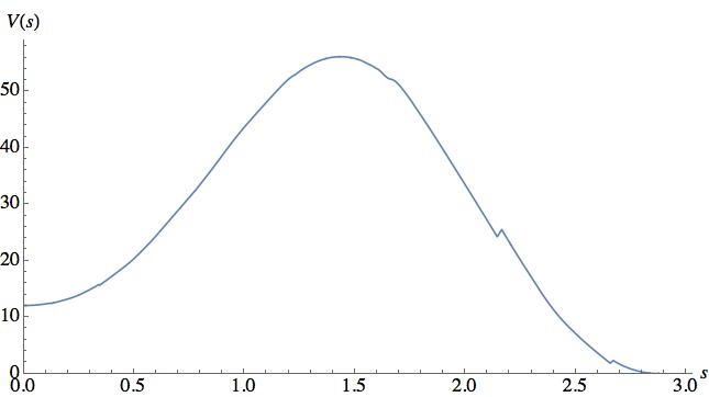
I'm getting inaccurate results when computing (plotting) the value of a function against the length of a line integral, where the path comes from a set of numerically calculated points. (In contrast, the integral seems fine when I have an analytic formula.)

For example: The matrix named points1 (which comes from stitching together a few numerical integrations, from NDSolve), composed of a few hundred real-valued triples, should define a smooth path (x(s),y(s),V(x(s),y(s))). I compute (interpolate) a parameterized line, and I plot the third component against the line integral of the first two components.

line1 = Table[ListInterpolation[points1[[1]][[All,jj]], {0,1}], {jj,1,3}]
ParametricPlot[{NIntegrate[Sqrt[line1[[1]]'[tt]^2+line1[[2]]'[tt]^2],{tt,0,ss}],
  line1[[3]][ss]}, {ss,0,1}]

In a few spots the vertical axis has small notches, i.e., changes of direction up and then down. The notches are small, but still visible. They are definitely spurious. I want to get five or so significant digits, and this is giving me three.

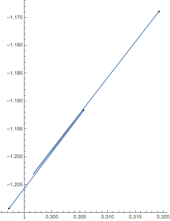
I think the problem might have to do with ListInterpolation giving changes in direction even when the set of points that it is interpolating is monotonic. I get the same problem whether I choose the method Spline or Hermite, and whichever method I give NIntegrate.

Suggestions, anyone?

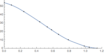
EDIT: Added code for one location where the problem shows up.

points = {
{0.6325952779137012, -0.7760085305401847, 54.07201697427571}, 
{0.62105807453548, -0.790281367826272, 53.57216747776533}, 
{0.5941956290244017, -0.8236073812563007, 52.209319984152756}, 
{0.5229935177928883, -0.9126291157398833, 47.34249397123951}, 
{0.3191937129061434, -1.1738845637283815, 26.841435108009442}, 
{0.30562102581445766, -1.1916609806787646, 25.358076396649462}, 
{0.2921897615948844, -1.2093010504444346, 23.900356246809537}, 
{0.2658926549639088, -1.243979893428035, 21.091685216353746}, 
{0.21635546253250398, -1.309812352799613, 16.05638285614679}, 
{0.13289109669708532, -1.422146100879459, 8.757698109321453}, 
{0.025168620642993245, -1.5688078584392655, 2.4156787966727435}, 
{0.020773587161218077, -1.5747852074054476, 2.2408427807381663}, 
{0.016541263234193266, -1.5805365848560005, 2.0788822741133828`}, 
{0.008539545100479554, -1.5913950062364555, 1.7898452227991974}, 
{-0.005774836825683922, -1.61075381814465, 1.328719820988212}, 
{-0.028775790485831575, -1.641584474796247, 0.7368957514090972}, 
{-0.03120754151431262, -1.644815864289341, 0.6849477369657428}, 
{-0.0335531257347027,-1.6479262887687476, 0.6367430278603834}, 
{-0.03799906267998585, -1.6538030044313163, 0.5504755732460467}, 
{-0.045993704234286795, -1.664298846988861, 0.41201122449151484}, 
{-0.058970977912545186, -1.681084608190775, 0.23202329470223404}
};

 line = Table[ ListInterpolation[points[[All, jj]], {0, 1}],  {jj, 1, 3} ];

 ParametricPlot[
   {
     NIntegrate[Sqrt[line[[1]]'[tt]^2 + line[[2]]'[tt]^2], {tt, 0, ss}],
     line[[3]][ss]
  },
       {ss, 0, 1},
   PlotRange -> {{0, All}, {0, All}},
   AspectRatio -> 1/2
       ]

Answer 1

The interpolation overshoots the next point and reverses direction.

ParametricPlot[{line[[1]][tt], line[[2]][tt]}, {tt, 0.2, 0.3}, 
 Epilog -> {Point[points[[All, 1 ;; 2]]]}]

You can reduce the interpolation order to 1 or use a centripetal parametrization parametrizeCurve from J.M.'s answer.

parametrizeCurve[pts_List, a : (_?NumericQ) : 1/2] := 
 FoldList[Plus, 0, Normalize[(Norm /@ Differences[pts])^a, Total]] /; 
  MatrixQ[pts, NumericQ]

tvals = parametrizeCurve[points];
line = Interpolation[Transpose[{tvals, #}]] & /@ Transpose@points;

s[t_?NumericQ] := 
  NIntegrate[Norm[{line[[1]]'[tt], line[[2]]'[tt]}], 
   Evaluate @ DeleteDuplicates @
     Flatten[{tt, 0, Select[tvals, 0 < # < t &], t}]];

ParametricPlot[
  Evaluate@{s[ss], line[[3]][ss]}, 
  {ss, 0, 1}, 
  PlotRange -> {{0, All}, {0, All}}, 
  AspectRatio -> 1/2, 
  Epilog -> {Point@Table[{s[ss], line[[3]][ss]}, {ss, 0, 1, 0.1}]}
]

Including the interpolation grid points tvals in NIntegrate speeds up the integration. For a really fast implementation use

s = NDSolveValue[{ss'[t] == Norm[{line[[1]]'[t],line[[2]]'[t]}], ss[0]==0}, ss, {t, 0, 1}]

which constructs an InterpolatingFunction for the arc length.