Can Reduce *really* not solve for x here?

Question

Sometimes I get the feeling I'm just flailing blindly with Mathematica. Is solving for $x$ in the equation $$ \frac{\cosh (x/2)}{x} = \sqrt{2} $$ really beyond the scope of Mathematica? I try to solve it with the command:

Reduce[(1/x)Cosh[x/2] == Sqrt[2], x]

and am met with

Reduce::nsmet: This system cannot be solved with the methods available to Reduce.

I get a feeling that I'm doing something very silly. Cheers for any assistance!

Answer 1

Use

Reduce[(1/x) Cosh[x/2] == Sqrt[2], x, Reals]

or

Solve[(1/x) Cosh[x/2] == Sqrt[2], x, Reals]

the latter yields

{{x -> Root[{-E^(-(#1/2)) - E^(#1/2) + 2 Sqrt[2] #1 &,      0.75858229952537718426}]}, 
 {x ->  Root[{-E^(-(#1/2)) - E^(#1/2) + 2 Sqrt[2] #1 &, 5.4693513860610533998}]}}

For transcendental equations you may get with Reduce or Solve roots represented symbolically by Root though they are in general transcendental numbers, so their values are written numerically beside the transcendental function written in the form of a pure function.

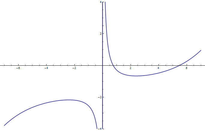
Plot[ (1/x) Cosh[x/2] - Sqrt[2], {x, -7, 7}, PlotStyle -> Thick, PlotRange -> {-4, 4}]

Edit

It should be emphasized that using domain specifications in Reduce or Solve you may still get messages of unsolvability of a given equation or a system (of eqations or/and inequalities), e.g.

Reduce[ x Cos[x/2] == Sqrt[2], x, Reals]

Reduce::nsmet: This system cannot be solved with the methods available to Reduce. >>
Reduce[x Cos[x/2] == Sqrt[2], x, Reals]

even though for a slightly different equation you can get the full solution, e.g.

Reduce[x Cos[x/2] == 0, x, Reals]

In these two cases there is an infinite number of solutions, but the latter case is much easier, because a solution satisfies one of the two conditions : x == 0 or Cos[x/2] == 0. In the first case we need to restrict a region where we'd like to find solutions. There we find all of them with Reduce (as well as with Solve) if in a given region there is only a finite number of solutions, e.g. restricting the domain to real numbers such, that -25 <= x <= 25 i.e. adding a condition -25 <= x <= 25 to a given equation (now we needn't specify explicitly the domain to be Reals because Reduce[expr,vars] assumes by default that quantities appearing algebraically in inequalities are real):

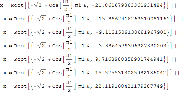
sols = Reduce[x Cos[x/2] == Sqrt[2] && -25 <= x <= 25, x]

Defining

f[x_] := x Cos[x/2] - Sqrt[2]

we can easily check that sols are indeed the solutions :

FullSimplify[ f[ sols[[#, 2]]]] & /@ Range @ Length[sols]

{0, 0, 0, 0, 0, 0, 0}

To extract only numerical values of the roots combined with zero we can do (see e.g. this answer):

Tuples[{List @@ sols[[All, 2, 1, 2]], {0}}]

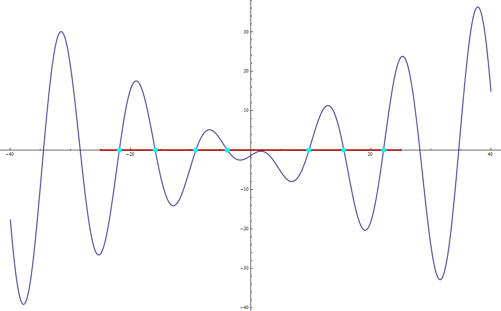
Now we can plot the function with appropriately marked roots and the specified domain :

Plot[ f[x], {x, -40, 40}, PlotStyle -> Thick, 
             Epilog -> {Thickness[0.003], Darker@Red, Line[{{-25, 0}, {25, 0}}], 
                        PointSize[0.01], Cyan, Point /@ Tuples[{List @@ sols[[All, 2, 1, 2]], {0}}]}]

Here the dark red line denotes the domain of our interest, and the cyan points denote all roots of the function f in this region.

Answer 2

All of these work:

f[x_] := Cosh[x/2]/x - Sqrt[2];

FindRoot      [f[x] == 0, {x, 1}]
N@FindInstance[f[x] == 0, x, Reals, 2]
N@Reduce      [f[x] == 0, x, Reals]
NSolve        [f[x] == 0, x, Reals]
N@Solve       [f[x] == 0, x, Reals]