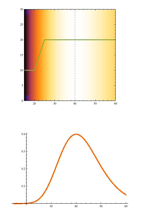
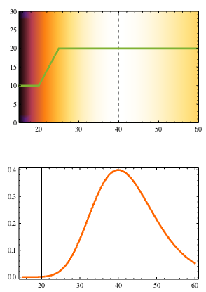
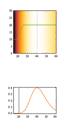
I am trying to show a gradient field behind a plot, and then its density in a separate plot below.
I understand (as in this question) that this must normally be done using the ImagePadding directive. However, that does not quite align the plots in this case:
padding = {{20, 30}, {20, 30}};
GraphicsColumn[
  {
   Show[
    DensityPlot[PDF[NormalDistribution[0, 1], Log[x/40]] ,
      {x, 15, 60}, {y, 0, 30},
      ColorFunction -> "SunsetColors"],
    Graphics[{Dashed, Gray, Line[{{40, 0}, {40, 30}}]}],
    Plot[If[x < 20, 10, If[x < 25, 2 x - 30, 20]], {x, 15, 60},
      PlotRange -> {0, 30} ,
      PlotStyle -> {RGBColor[0.5, .7, 0.2], Thickness[0.01]}],
    ImagePadding -> padding, PlotRangePadding -> None
   ],
   Plot[PDF[NormalDistribution[0, 1], 5 Log[x/40]] , {x, 15, 60},
      PlotStyle -> {RGBColor[1, 0.4, 0], Thickness[0.01]},
      ImagePadding -> padding]
  }
]

Is there a way to get the abscissa ranges to match?


PlotRangeexplicitly for both plots $\endgroup$