1
$\begingroup$

I have the following data

data={{1.5, 10}, {25, 26.5}, {29.25, 32.75}, {39.25, 42.5}, {62.5, 67}, {73.5, 80.75}, {87.5, 93}, {102, 104.75}, {111, 114.5}, {123, 129}, {146.5, 152.75}, {161.5, 164.5}, {177, 182.25}, {195.75, 206}, {218.25, 226.25}, {234.75, 237.75}, {246, 252.5}, {258.5, 260.25},{266.25, 272.75}, {280.5, 280.75}, {281.5, 283}, {292,301.25}, {314, 322}, {327.5, 328.5}, {329, 330.25}}

Each set of point denotes the starting and ending point of the pulse, so here there are as many pulses as

Length[data]

I make the function consisting of all these pulses as follows:

f[x_] := Sum[HeavisideTheta[x - Part[data, i, 1]] + HeavisideTheta[-x+Part[data,i,2]], {i, 1, Length[data]}]

This - as it can be checked - uses 2 Heaviside functions to create each pulse. The problem is while plotting the net pulse function:

Plot[f[x], {x, 0, Part[Last[data], 2] + 10}, Filling -> Bottom]
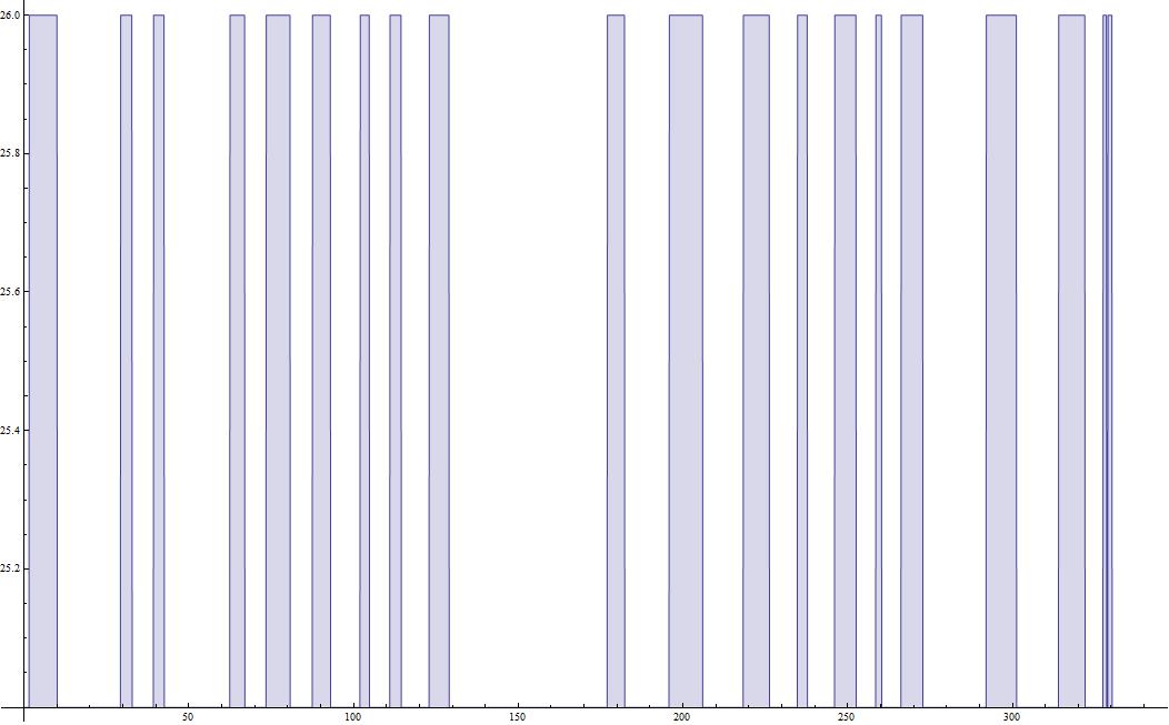
enter image description here

As it can be seen from the "data" list, there are supposed to be the

{146.5, 152.75}, {161.5, 164.5} and {280.5, 280.75}, {281.5, 283}

pulses in the plot that are just missing.

I just can't figure out how this is happening. Any help will be greatly appreciated!

$\endgroup$
3

2 Answers 2

3
$\begingroup$

Artes's solution is the most general one that works for numerical black box functions as well.

In this special case however, we have a different option: make sure that Plot sees the expression of the function. It will recognize HeavisideTheta as a function with a discontinuity, and it will plot the discontinuities as their precise location (not at a numerical approximation of this location, found using Plot's adaptive sampler).

Let's define f like this:

Clear[f, x]
f[x_] = Sum[HeavisideTheta[x - p[[1]]] + HeavisideTheta[-x + p[[2]]], {p, data}]

Make sure to use = instead of := to build the complete symbolic function.

Now let's plot as

Plot[f[x], {x, 0, data[[-1, 2]] + 10}, Filling -> Bottom, ExclusionsStyle -> Automatic]

ExclusionsStyle -> Automatic means: use the same line style for the discontinuities as for the rest of the plot.

Notice that this plots all the discontinuities, but some of the fillings are missing. To get those as well, we still need to increase the plot points:

Plot[f[x], {x, 0, data[[-1, 2]] + 10}, Filling -> Bottom, ExclusionsStyle -> Automatic, PlotPoints -> 100]

But at least it is guaranteed that all the discontinuities will be found without needing to use a high PlotPoints and any MaxRecursion settings. The manual PlotPoints setting is only to make sure that the fillings are all present as well.

Reference: http://reference.wolfram.com/mathematica/ref/Exclusions.html

$\endgroup$
1
$\begingroup$

As Artes noted, adding to Plot e.g. these options resolves the problem:

PlotPoints -> 200, MaxRecursion -> 4
$\endgroup$

Your Answer

By clicking “Post Your Answer”, you agree to our terms of service and acknowledge you have read our privacy policy.

Not the answer you're looking for? Browse other questions tagged or ask your own question.