How to get the steady-state analytical solution of a set of nonlinear differential equations?

Question

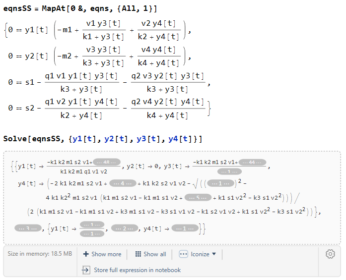
A paper I am reading recently studies a system with 4 variables shown in the picture. The authors showed how the ratio of X_pro and X_syn would change over different parameters at steady state. According to the authors, they solved the equations at steady state using Mathematica . But I am not sure how to do that. (the paper can be accessed here https://journals.asm.org/doi/10.1128/spectrum.04000-22)

I tried this code:

eqns = {
y1'[t]==(v1*y3[t]/(y3[t]+k1)+v2*y4[t]/(y4[t]+k2)-m1)*y1[t], 
y2'[t]==(v3*y3[t]/(y3[t]+k3)+v4*y4[t]/(y4[t]+k4)-m2)*y2[t], 
y3'[t]==- v1*y3[t]/(y3[t]+k3)*q1*y1[t]-v3*y3[t]/(y3[t]+k3)*q2*y2[t]+s1,
y4'[t]==- v2*y4[t]/(y4[t]+k2)*q1*y1[t]-v4*y4[t]/(y4[t]+k4)*q2*y2[t]+s2
};
sol=DSolve[eqns,{y1,y2,y3,y4},t]

But I didn't get any results. So I wonder if anyone could help me with it. Thank you!

Answer 1

A steady-state is a condition in which the concentrations do not change anymore. This means that $$\frac{\mathrm{d}[X]}{\mathrm{d}t} = 0$$ for every component $X$.

Let's first change your equations to set y1'[t] == y2'[t] == y3'[t] == y4'[t] == 0:

eqnsSS = MapAt[0 &, eqns, {All, 1}];

Now we can use Solve to get the result.

sol = Solve[eqnsSS, {y1[t], y2[t], y3[t], y4[t]}]

Beware, it took a few minutes on my computer to get the result. There are 5 distinct sets of solution.

Answer 2

The steady state solution is a solution, where all functions become constant.

That is, all y' are to be set to zero

While the standard routines like Solve, Reduce, Eliminate are going to run endlessly, the standard elimination procedure is producing results.

Take the right hand sides and remove the argument [t]

  rhs = {(v1*y3[t]/(y3[t] + k1) + v2*y4[t]/(y4[t] + k2) - m1) ,
          (v3*y3[t]/(y3[t] + k3) + v4*y4[t]/(y4[t] + k4) - m2) , 
         -v1*y3[t]/(y3[t] + k3)*q1*y1[t] - v3*y3[t]/(y3[t] +
            k3)*q2*y2[t] + s1, 
          -v2*y4[t]/(y4[t] + k2)*q1*y1[t]-v4*y4[t]/(y4[t]+ k4)*
             q2*y2[t] + s2} /. 
               {f_[t] :> f};

and solve and eliminate for the y's backward, applying Numerator@Together in each stage

    eqn = (Numerator@Together[rhs] // FullSimplify);

    sl[4] = Solve[0 == eqn[[4]], y4][[1]] // FullSimplify

$$\left\{\text{y4}\to \frac{\sqrt{(\text{k2} (\text{s2}-\text{q2} \text{v4} \text{y2})+\text{k4} (\text{s2}-\text{q1} \text{v2} \text{y1}))^2+4 \text{k2} \text{k4} \text{s2} (\text{q1} \text{v2} \text{y1}+\text{q2} \text{v4} \text{y2}-\text{s2})}+\text{k2} \text{q2} \text{v4} \text{y2}-\text{k2} \text{s2}+\text{k4} \text{q1} \text{v2} \text{y1}-\text{k4} \text{s2}}{2 (-\text{q1} \text{v2} \text{y1}-\text{q2} \text{v4} \text{y2}+\text{s2})}\right\}$$

 eqn1 = eqn /. sl[4] // Together // Numerator // FullSimplify;

  sl[3] = Solve[0 == eqn1[[3]], y3][[1]] 

$$\left\{\text{y3}\to -\frac{\text{k3} \text{s1}}{-\text{q1} \text{v1} \text{y1}-\text{q2} \text{v3} \text{y2}+\text{s1}}\right\}$$

     eqn2 = eqn /. Join[sl[4], sl[3]] // Together // Numerator;

    Solve[0 == eqn2[[2]], y2] // Simplify;

     ((eqn /. {sl[4]} // Together // Numerator) /. {sl[3]} // 
   Together //  Numerator) /. 
   {sl[2][[1]]} // Together // Numerator // Simplify // PowerExpand

       {{{{0, 0, 0, 0}}}}

Answer 3

It's not often there's a question on here about resource competition of phytoplankton (my niche speciality), so I'm obligated to attempt an answer.

First, define the right-hand sides:

Clear["Global`*"]

dy1 = (v1*y3/(y3 + k1) + v2*y4/(y4 + k2) - m1)*y1;
dy2 = (v3*y3/(y3 + k3) + v4*y4/(y4 + k4) - m2)*y2;
dy3 = -v1*y3/(y3 + k3)*q1*y1 - v3*y3/(y3 + k3)*q2*y2 + s1;
dy4 = -v2*y4/(y4 + k2)*q1*y1 - v4*y4/(y4 + k4)*q2*y2 + s2;

Usually one would Solve for all of these equal to zero simultaneously as in @Domen's answer, but the expressions are complicated and there are many equilibria (since both species y1 and y2 could be present or absent). One trick is to divide their equations by yi to focus on the case of coexistence. They are still too ugly to look at, so I suppress output with a semicolon, but we can see that there are two of them:

eq = Solve[{dy1/y1 == 0, dy2/y2 == 0, dy3 == 0, dy4 == 0}, {y1, y2, y3, y4}];
Length[eq]
(* 2 *)

Alternatively, one could break it into two subproblems taking advantage of the fact that the species' per capita growth depends only on the nutrient concentrations (y3 and y4). This is why zero-net growth isoclines (ZNGIs) work in resource competition theory.

First, solve for nutrients when both species don't grow:

nuteq = FullSimplify[Solve[{dy1 == 0, dy2 == 0}, {y3, y4}]]
(* two not TOO ugly expressions *)

Then solve for species abundances when resources don't change:

speq = FullSimplify[Solve[{dy3 == 0, dy4 == 0}, {y1, y2}]][[1]]
(* one almost nice looking expression *)

I gather from the authors' python code (files s001_00_12_Optimized.py and Solutions01.py), this is what they did.

Finally, assign parameters and plot. Here's my attempt at Fig. 5A:

v1 = 1.14; v2 = 2.42; v3 = 2.17; v4 = 3.98;
k1 = 35.5; k2 = 11.8; k3 = 19.9; k4 = 69.2;
m1 = 0.706; m2 = 0.517;
q1 = 1.2*10^-4; q2 = 2.88*10^-4;
s2 = 0.005*10^3;
s1 := s2*sratio; (* define s1 in terms of s2 *)

LogLogPlot[Evaluate[(y1*q1/(y2*q2)) /. eq[[2]]], {sratio, 10^-1.5, 10^0.5}, PlotRange -> {{10^-1.5, 10^0.5}, {10^-4, 10^4}}]

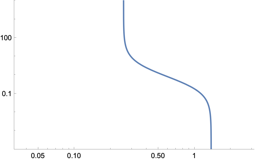
Looks pretty close, but might be off since you used different notation than in the paper. Also, I had to guess that eq[[2]] was the correct solution.

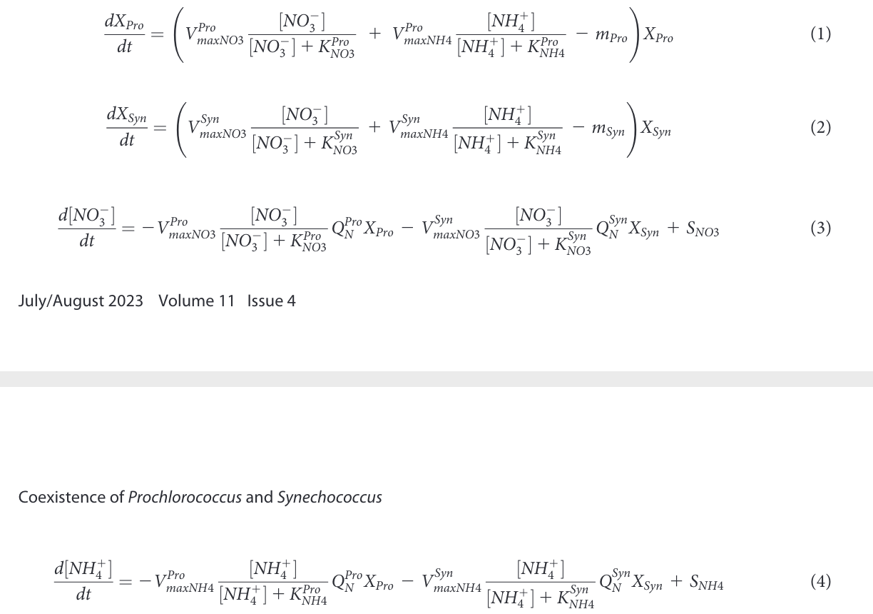
One other thing I can note: Replicating Fig. 2 requires a little hack to keep nutrient levels non-negative, due to the non-physical negative "source" terms as found in Table S4 of the Supplemental Material.