Response to OP's last edit:
[...] is it possible to add some kind of constraint to the Plot3D function, such that it only visualizes the actual function? [...]
It is visualising actual function. From Piecewise documentation you will get that it is by default set to 0 to other arguments than matched True with conditions. You can set B11[x_, y_] = Piecewise[{{1, 0 <= x <= 1 && 0 <= y <= 1}},None]; but unfortunatell it will get dirty after differentiation.
Lets assume you do not want to know specific coordinates but only plot the wireframe you've described.
I'm going to put with force None to last part of B111. Then we will use BoundaryStyle and ExlusionsStyle to plot the wireframe ;)
 B11[x_, y_] = Piecewise[{{1, 0 <= x <= 1 && 0 <= y <= 1}}];
 B111[x_, y_] = Integrate[B11[x - t, y - t], {t, 0, 1}];

 f[x_, y_] = Piecewise[First[List @@ B111[x, y]], None]

 Plot3D[f[x, y], {x, -0.2, 2.2}, {y, -0.2, 2.2}, Axes -> False, Mesh -> None,
                 ExclusionsStyle -> Directive[Thick, Red], PlotStyle -> None,
                 BoundaryStyle -> Directive[Thick, Red], Boxed -> False,
                 Lighting -> "Neutral", ImageSize -> 500]
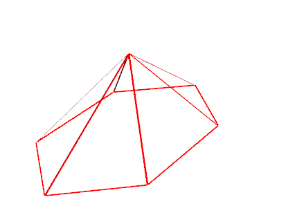
Accurate approach
We will take only what we need to. ;)
following function replaces inequalities with equalities and looks for "convex hull" minimal sample of critical points of the region.
In this simple case (triangles) they can be used straightforwardly to create regions. for more complex regions it will require deeper analysis.
pointExtract[cond_] := Module[{ineq = {Less, LessEqual, GreaterEqual, Greater}, temp},
           temp = LogicalExpand@cond; (*<- important part, thanks to halirutan's
                                        important remarks*)
           temp = (temp /. {f_[x__, a__] :> Equal[x, a] /; MemberQ[ineq, f],
                            And -> Or}
                  ) /. Or -> List; (*making equalities*)
           temp = Tuples[temp, 2]; (*pairing them to each other*)
           DeleteDuplicates@Cases[{x, y} /. ((Quiet@Solve[#, {x, y}] & /@ temp)),
                                  {_?NumericQ ..}, \[Infinity]] (*solving paired equations*)
                    ]
Now we have to prepare set of inequalities:
eq = (List @@ B111[x, y])[[1, ;; , 2]] /. Or -> Sequence

points = DeleteCases[pointExtract /@ eq, {Repeated[{_, _}, 2]}];
(*we only take those with 3 or more points since we are not interested in lines and points*)
Graphics[{Hue@RandomReal[], Polygon[#]} & /@ points] (*domains plot*)
Below I have assumed that additional point is {1, 1, 1} (from B111 form) but it can be easily generalised.
Graphics3D[With[{len = Length@#},
GraphicsComplex[
         ({##, 0} & @@@ #)~Join~{{1, 1, 1}},
         {Hue@RandomReal[], [email protected],
          Line[{##, len + 1} & @@@ Partition[{Sequence @@ Range[len], 1}, 2, 1]]}]
               ] & /@ points

          , Boxed -> False]
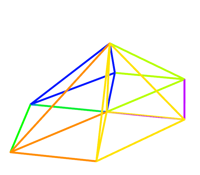
First, not accurate approach
The question is: how much do you need to know about those borders.
If you just want to plot the regions the following method is simple enough:
eq = (List @@ B111[x, y])[[1, ;; , 2]]

RegionPlot[eq, {x, -.1, 2.2}, {y, -.1, 2.2}, PlotPoints -> 50, PlotStyle -> None,
                                             BoundaryStyle -> Blue]
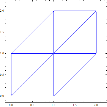
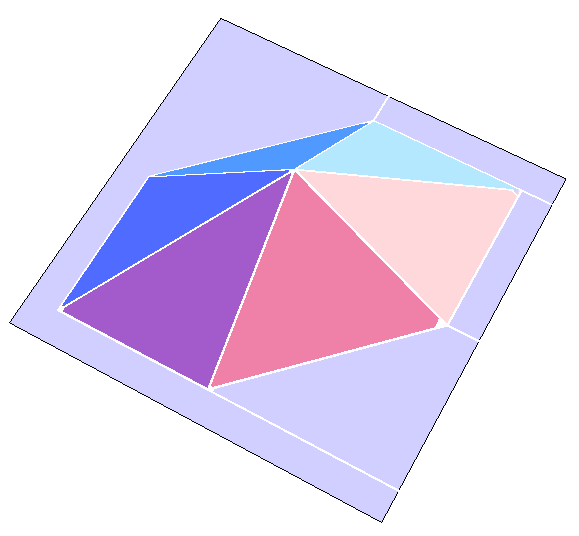
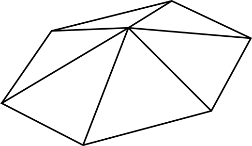


Plot3D[..., Exclusions -> None]]. For a better resolution use higher values ofPlotPointsandMaxRecursion, e.gPlotPoints -> 50, MaxRecursion -> 4. $\endgroup$