8
$\begingroup$

I'm wondering how to display the support $\mathrm{supp}(f)$ of a piecewise surface $z = f(x,y)$.

As an example, let's consider the following piecewise function (and plot it):

f[x_, y_] = Piecewise[{{1, 0 <= x <= 1 && 0 <= y <= 1}}];
g[x_, y_] = Integrate[f[x - t, y - t], {t, 0, 1}];
Plot3D[g[x, y], {x, -0.5, 2.5}, {y, -0.5, 2.5}, PlotRange -> Full]
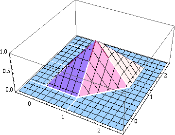
plot of example function

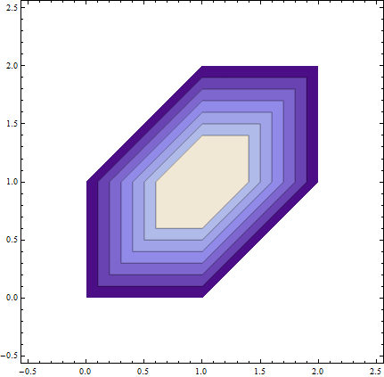
My first thought was to use a contour plot for this purpose, such as

ContourPlot[g[x, y] == .05, {x, -0.5, 2.5}, {y, -0.5, 2.5}]
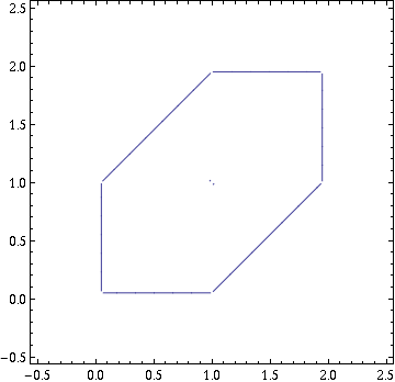
the contour plot

But this is of course only an approximation of the support. How do I display the actual support of my piecewise function?

Edit

The proposed solution in the comments below works great, the result looks as follows:
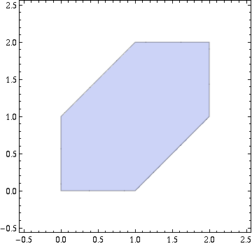
plot of the region

$\endgroup$
3
  • 2
    $\begingroup$ Something like RegionPlot[Or @@ Most[First[Internal`FromPiecewise[g[x, y]]]] // Evaluate, {x, -0.5, 2.5}, {y, -0.5, 2.5}]? $\endgroup$ Commented Jun 19, 2013 at 9:59
  • 2
    $\begingroup$ RegionPlot[ g[x, y] > 0, {x, -0.5, 2.5}, {y, -0.5, 2.5}] $\endgroup$
    – Artes
    Commented Jun 19, 2013 at 10:00
  • $\begingroup$ Thanks! Didn't know about this option, it works great. $\endgroup$
    – Ailurus
    Commented Jun 19, 2013 at 10:06

2 Answers 2

11
$\begingroup$

The most direct way uses RegionPlot e.g.

RegionPlot[ g[x, y] > 0, {x, -0.5, 2.5}, {y, -0.5, 2.5}]

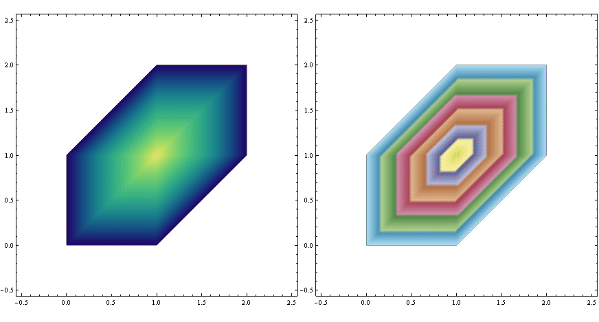
let's customize it a bit using colors from many possible ColorData["Gradients"]:

GraphicsRow[ 
    RegionPlot[ g[x, y] > 0, {x, -0.5, 2.5}, {y, -0.5, 2.5}, 
                ColorFunction -> Function[{x, y}, ColorData[#][Abs[g[x, y]]]], 
                ColorFunctionScaling -> False, PlotPoints -> 100, MaxRecursion -> 5]& /@
    {"BlueGreenYellow", "DarkBands"} ]

enter image description here

One can also get the plot with ContourPlot, e.g. using the RegionFunction option:

ContourPlot[ g[x, y], {x, -0.5, 2.5}, {y, -0.5, 2.5}, 
             RegionFunction -> Function[{x, y}, g[x, y] > 0], Exclusions -> None] 

enter image description here

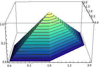
At last, we can make Plot3D better fitting to our needs:

Plot3D[ g[x, y], {x, -0.5, 2.5}, {y, -0.5, 2.5}, MeshFunctions -> {#3 &}, 
        PlotRange -> All, RegionFunction -> Function[{x, y}, g[x, y] > 0], 
        ColorFunction -> Function[{x, y}, ColorData["BlueGreenYellow"][g[x, y]]], 
        ColorFunctionScaling -> False, BoxRatios -> {2, 2, 1}, PlotPoints -> 80, 
        MaxRecursion -> 4, Exclusions -> None]

enter image description here

$\endgroup$
12
$\begingroup$

Here's another quick way to visualize the support region:

RegionPlot[Or @@ g[x, y][[1, All, 2]] // Evaluate, {x, -0.5, 2.5}, {y, -0.5, 2.5}]

support region for a piecewise function.

In some cases, one might want to run Reduce[] on the pile of constraints produced by Or @@ g[x, y][[1, All, 2]], before plotting, to reduce evaluation effort. (In this case, it did not do much, but it's a good idea in general.)

If one is not afraid of undocumented functions, here is another method:

RegionPlot[Or @@ Most[First[Internal`FromPiecewise[g[x, y]]]] // Evaluate,
           {x, -0.5, 2.5}, {y, -0.5, 2.5}]
$\endgroup$
0

Your Answer

By clicking “Post Your Answer”, you agree to our terms of service and acknowledge you have read our privacy policy.

Not the answer you're looking for? Browse other questions tagged or ask your own question.