How do I construct and plot functions properly using NestList?

Question

I am trying to construct a function using NestList and plot the values. Although the individually used and defined functions in my notebook seem to do the right thing (have compared the outputs with an equivalent Python notebook), I am failing at the procedure. In particular, the performance is very poor, but this must be due to my implementation.

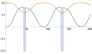
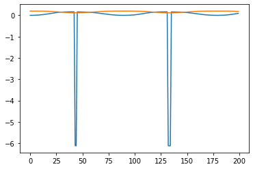
Background: The idea is to investigate error propagation function of qubit rotations (using $SU2$ rotations). Using Mathematica, I plan to use CAS features like simplifications or determining curve equations. The following plot shows the angular error after $n$ rotations of a qubit on the bloch sphere:

The corresponding Python Code looks as follows:

rot_x = pi/100
rot_y = pi/100
rot_z = pi/100
num_iterations = 200

start_vec = [1, 0, 0]
err = 0.2

x = np.arange(0, num_iterations, 1, dtype=int)
ϕ_error_propagation_vec = np.zeros(shape=(num_iterations))
θ_error_propagation_vec = np.zeros(shape=(num_iterations))

vec = start_vec
vec_err = qubitmatrix_to_cartesian(rn_su2_euler(start_vec, 0, err, 0))

for i in range(num_iterations):    
    polar = cartesian_to_spherical(vec)
    polar_err = cartesian_to_spherical(vec_err)
    (ϕ_rotated, θ_rotated) = (polar[1], polar[2])
    (ϕ_rotated_err, θ_rotated_err) = (polar_err[1], polar_err[2])

    θ_error_propagation_vec[i] = θ_rotated_err - θ_rotated
    ϕ_error_propagation_vec[i] = ϕ_rotated_err - ϕ_rotated

    M_q_rotated = rn_su2_euler(vec, rot_x, rot_y, rot_z)
    M_q_rotated_err = rn_su2_euler(vec_err, rot_x, rot_y, rot_z)
    vec = qubitmatrix_to_cartesian(M_q_rotated)
    vec_err = qubitmatrix_to_cartesian(M_q_rotated_err)

plt.plot(x, ϕ_error_propagation_vec, θ_error_propagation_vec)
plt.show()

For the sake of completeness, I provided the whole working Notebook including all functions here on GitHub.

My question and approach: I reimplemented this script using Mathematica (v.13) as follows:

ClearAll["Global`*"];
qubitmatrixToCartesian[Mq_] := (
   q1 = Re[(Mq[[1, 2]] + Mq[[2, 1]])/2];
   q2 = Re[(Mq[[2, 1]] - Mq[[1, 2]])/(2*I)];
   q3 = Re[Mq[[1, 1]]];
   Return[{q1, q2, q3}];
   );
rnSU2euler[vec_, rx_, ry_, rz_] := (
   sphericalVec = ToSphericalCoordinates[vec];
   \[Theta] = sphericalVec[[2]];
   \[Phi] = sphericalVec[[3]];
   sx = PauliMatrix[1];
   sy = PauliMatrix[2];
   sz = PauliMatrix[3];
   Mq = Sin[\[Theta]]*Cos[\[Phi]]*sx + Sin[\[Theta]]*Sin[\[Phi]]*sy + 
     Cos[\[Theta]]*sz;
   Un = {{Exp[-I*(rx + rz)/2]*Cos[ry/2], -Exp[-I*(rx - rz)/2]*
       Sin[ry/2]}, {Exp[I*(rx - rz)/2]*Sin[ry/2], 
      Exp[I*(rx + rz)/2]*Cos[ry/2]}};
   Return [Un . Mq . ConjugateTranspose[Un]];
   );
rotateVector[vec_, rx_, ry_, rz_] := (
   MqRotated = rnSU2euler[vec, rx, ry, rz];
   Return[qubitmatrixToCartesian[MqRotated]];
   );
errorPropagation[n_, vec_, vecError_, rx_, ry_, rz_] := (
   v = N[NestList[rotateVector[#, rx, ry, rz] &, vec, n]];
   vErr = N[NestList[rotateVector[#, rx, ry, rz] &, vecError, n]];
   polar = Map[ToSphericalCoordinates, v];
   polarErr = Map[ToSphericalCoordinates, vErr];
   Return[MapThread[Subtract, {polar[[All, 2]], polarErr[[All, 2]]}]];
   );
ListPlot[errorPropagation[4, {1, 0, 0}, 
  N[rotateVector[{1, 0, 0}, 0, 0.02, 0]], Pi/100, Pi/100, Pi/100]]

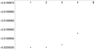
Unfortunately, the performance drops (the scripts hangs) after drawing 5 values. I strongly suspect that the function errorPropagation is implemented improperly:

The values seem to be plausible, and the individual functions work well. But I am doing at least something wrong with the way I am using NestList. I would be greatful for any help to get my script plotting the curves as depicted by the figure shown further above.

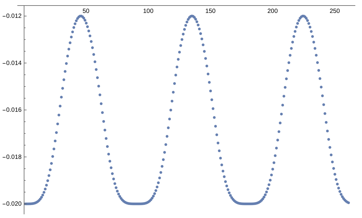
Update (2022-06-25): Following the straight-forward answer given by MarcoB I could generate the desired chart:

Answer 1

Since the ultimate purpose appears to be plotting, and since your code is already interspersed with calls to N, numerical results appear to be OK.

One problem is, however, that those calls to N are "too late", that is they appear after the expensive calculations have already been done symbolically. If you can get away with, it is always better for performance to start out with machine-precision results instead.

Below is a reformatted version of your code that easily handles a few hundred points essentially just by adding N before the expensive calculations rather than after.

I also got rid of the Return calls (you almost never need those: functions in MMA return the last value they calculate), and encapsulated each function body in a Module to localize variables. Note also that you don't need MapThread to do element-wise subtraction between two lists; you can just write polar[[All, 2]] - polarErr[[All, 2]].

ClearAll["Global`*"]

qubitmatrixToCartesian[Mq_] := Module[{q1, q2, q3},
   q1 = Re[(Mq[[1, 2]] + Mq[[2, 1]])/2];
   q2 = Re[(Mq[[2, 1]] - Mq[[1, 2]])/(2*I)];
   q3 = Re[Mq[[1, 1]]];
   {q1, q2, q3}
  ]

rnSU2euler[vec_, rx_, ry_, rz_] := Module[{sphericalVec, \[Theta], \[Phi], sx, sy, sz, Mq, Un},
   sphericalVec = ToSphericalCoordinates[vec];
   \[Theta] = sphericalVec[[2]];
   \[Phi] = sphericalVec[[3]];
   sx = PauliMatrix[1];
   sy = PauliMatrix[2];
   sz = PauliMatrix[3];
   Mq = Sin[\[Theta]]*Cos[\[Phi]]*sx + Sin[\[Theta]]*Sin[\[Phi]]*sy + 
     Cos[\[Theta]]*sz;
   Un = {{Exp[-I*(rx + rz)/2]*Cos[ry/2], -Exp[-I*(rx - rz)/2]*
       Sin[ry/2]}, {Exp[I*(rx - rz)/2]*Sin[ry/2], 
      Exp[I*(rx + rz)/2]*Cos[ry/2]}};
   Un . Mq . ConjugateTranspose[Un]
 ]

rotateVector[vec_, rx_, ry_, rz_] := Module[{MqRotated},
   MqRotated = rnSU2euler[vec, rx, ry, rz];
   qubitmatrixToCartesian[MqRotated]
 ]

errorPropagation[n_, vec_, vecError_, rx_, ry_, rz_] := Module[{v, vErr, polar, polarErr},
   v = NestList[rotateVector[#, rx, ry, rz] &, N@vec, n];
   vErr = NestList[rotateVector[#, rx, ry, rz] &, N@vecError, n];
   polar = Map[ToSphericalCoordinates, v];
   polarErr = Map[ToSphericalCoordinates, vErr];
   polar[[All, 2]] - polarErr[[All, 2]]
 ]
   
ListPlot[
  errorPropagation[
    260, 
    {1, 0, 0}, 
    rotateVector[{1, 0, 0}, 0, 0.02, 0],
    Pi/100, Pi/100, Pi/100
  ]
]