Plotting fractals in Mathematica for S iteration

Question

Dears, I'm trying to plot the attached picture figures in Mathematica software.

Let $T(z)=z-\frac{P(z)}{P^{\prime}(z)}$. The S iterative scheme is for $z_{0}$ a starting point and $y_{n}=(1-\beta_{n})z_{n}+\beta_{n}Tz_{n}$, $z_{n+1}=(1-\alpha_{n})Tz_{n}+\alpha_{n}Ty_{n}$, n=0,1,2,....

Now if $P(z)=z^{3}-1$ and considered the square domains centered at the origin in the complex plane $D=[-2,2]\times[-2,2]$ and To generate the basins of attraction and to study the behaviors of Mann iteration procedure, we take the corresponding square domain and divide it into $250\times 250$ grids. By using Newton’s operator N(z), we generate the sequence $\{z_{n}\}$; n = 1; 2; 3; corresponding to an iteration procedure, starting at each grid point z0. If the sequence $\{z_{n}\}$; n = 1; 2; 3; attempt a root of a polynomial with the accuracy of $10^{-4}$ in a $k \leq 13$ number of iterations, then the converging point $z_0$ is colored in a color assigned to k, otherwise the point is colored in white. The fig (b) obtain fig if $\alpha_{n}=\beta_{n}=0.9$. The complete paper is free to download at https://www.researchgate.net/publication/307016155_A_comparison_of_some_fixed_point_iteration_procedures_by_using_the_basins_of_attraction

I have tried the code in Mathematica but can not find any images like this.

P[z_] := z^3 - 1;
T[z_] := z - (T[z]/T'[z]);
α[n_] := 0.9;
β[n_] := 0.9;
z[0] = AnyTrue;
y[n_] := (1 - β[n])*z[n] + β[n]*T[z[n]];
z[n_] := (1 - α[n - 1])*T[z[n - 1]] + α[n - 1]*T[y[n - 1]];

Answer 1

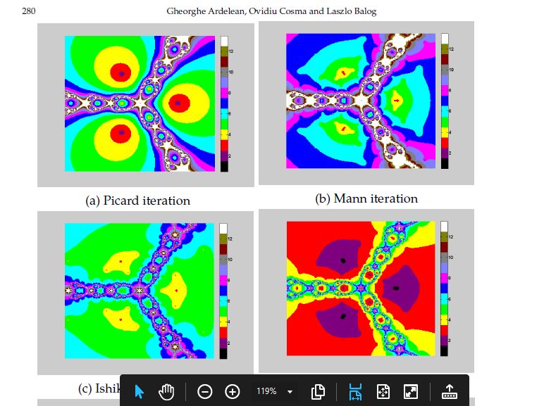
Implementing this in Mathematica is not difficult. Lets start by implementing some iteration operators (the interested reader might add additional operators from the paper):

ClearAll[Tnewton,Tmann,Tkahn,TM]
Tnewton[P_,dPdz_]:=Module[{x,n},Inactive[Function][{x,n},x-P[x]/dPdz[x]]//Activate]
Tmann[alpha_][P_,dPdz_]:=Module[{x,n},Inactive[Function][{x,n},(1-alpha[n])x+alpha[n] Tnewton[P,dPdz][x,0]]//Activate]
Tkahn[alpha_][P_,dPdz_]:=Module[{x,n},Inactive[Function][{x},With[{y=(1-alpha[n])x+alpha[n] Tnewton[P,dPdz][x,0]},Simplify@Tnewton[P,dPdz][y,0]]]//Activate]
TM[alpha_][P_,dPdz_]:=Module[{x,n},Inactive[Function][{x},With[{y=(1-alpha[n])x+alpha[n] Tnewton[P,dPdz][x,0]},Simplify@Tnewton[P,dPdz][Tnewton[P,dPdz][y,0],0]]]//Activate]

These functors generate iteration functions after providing the polynomial, its derivative and optional parameters.

We continue by defining some test function, its derivative, resulting iterators and its roots:

P3=Function[{z},z^3-1];
dP3dz=Module[{z},Inactive[Function][{z},D[P3[z],z]]//Activate];
P3Tnewton=Tnewton[P3,dP3dz];
P3Tmann=Tmann[0.9&][P3,dP3dz];
P3Tkahn=Tkahn[0.9&][P3,dP3dz];
P3TM=TM[0.9&][P3,dP3dz];
P3roots=Solve[P3[z]==0,z][[All,1,2]];

P5=Function[{z},z^5+z^4+z^3+z^2+z];
dP5dz=Module[{z},Inactive[Function][{z},D[P5[z],z]]//Activate];
P5Tnewton=Tnewton[P5,dP5dz];
P5Tmann=Tmann[0.9&][P5,dP5dz];
P5Tkahn=Tkahn[0.9&][P5,dP5dz];
P5TM=TM[0.9&][P5,dP5dz];
P5roots=Solve[P5[z]==0,z][[All,1,2]];

The main iteration routine to compute the basins of attraction is

iteration[T_,Proots_,nmax_:13,epsilon_:10^-4,printQ_:False][z_]:=Module[{it,n,itn},
  it[0]=z;
  it[n_]:=it[n]=T[it[n-1],n];
  n=0;
  While[n<=nmax,
    itn=it[n];
    If[printQ,Print[{n,itn,Abs[itn-#]&/@Proots}]];
    If[Min[Abs[itn-#]&/@Proots]<epsilon,Return[n];];
    n++;
  ];
  Return[-1];
]

This function returns $-1$ if the iteration fails to converge (up to a absolute precision epsilon) to one of the specified roots in the specified number of maximal iterations nmax. If the iteration converges the number of iteration steps n is returned.

Now we can generate some plots using

m=250;
aRange=Subdivide [-2.,2.,m];
bRange=aRange;

P3newton=Quiet@ParallelTable[{a,b,Quiet@iteration[P3Tnewton,P3roots,13][a+I b]},{a,aRange},{b,bRange},DistributedContexts->All];
P3mann=Quiet@ParallelTable[{a,b,Quiet@iteration[P3Tmann,P3roots,13][a+I b]},{a,aRange},{b,bRange},DistributedContexts->All];
P3khan=Quiet@ParallelTable[{a,b,Quiet@iteration[P3Tkahn,P3roots,13][a+I b]},{a,aRange},{b,bRange},DistributedContexts->All];
P3M=Quiet@ParallelTable[{a,b,Quiet@iteration[P3TM,P3roots,13][a+I b]},{a,aRange},{b,bRange},DistributedContexts->All];

ClearAll[m,aRange,bRange];

colorFuntion=Function[{k},If[k<0||k>13,White,{RGBColor[0.001,0.001,0.001],RGBColor[0.001,0.001,0.001],RGBColor[0.494,0.001,0.494],RGBColor[0.994,0.007,0.001],RGBColor[0.992,0.993,0.001],RGBColor[0.012,0.995,0.002],RGBColor[0.001,0.993,0.992],RGBColor[0.013,0.006,0.995],RGBColor[0.991,0.001,0.994],RGBColor[0.497,0.5,0.995],RGBColor[0.496,0.495,0.494],RGBColor[0.499,0.003,0.002],RGBColor[0.5,0.5,0.001],RGBColor[1.,1.,1.]}[[Floor[k]+1]]]];

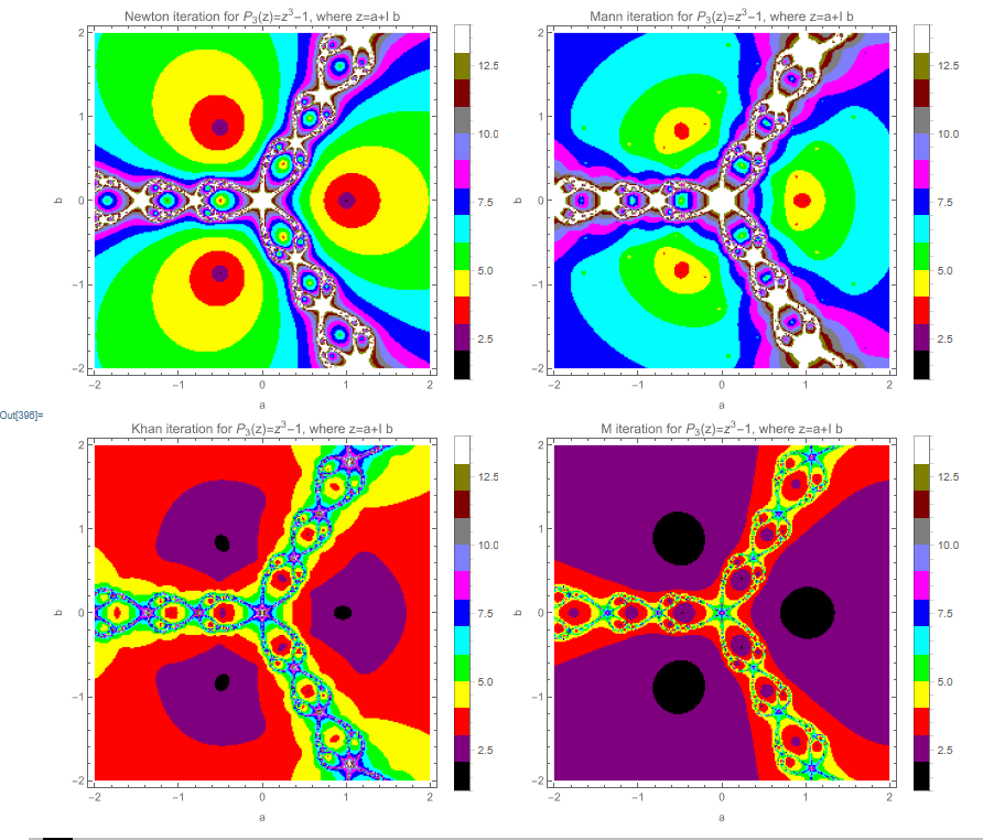
plot=ListDensityPlot[Flatten[#1,1],PlotLegends->Placed[BarLegend[{colorFuntion,{1,14}}],Right],InterpolationOrder->0,PlotRange->All,ColorFunction->colorFuntion,ColorFunctionScaling->False,FrameLabel->{"a","b"},PlotLabel->#2<>" iteration for Subscript[P, 3](z)=z^3-1, where z=a+I b",ImageSize->350]&;
Grid[{{plot[P3newton,"Newton"],plot[P3mann,"Mann"]},{plot[P3khan,"Khan"],plot[P3M,"M"]}}]
Clear[plot]

resulting in

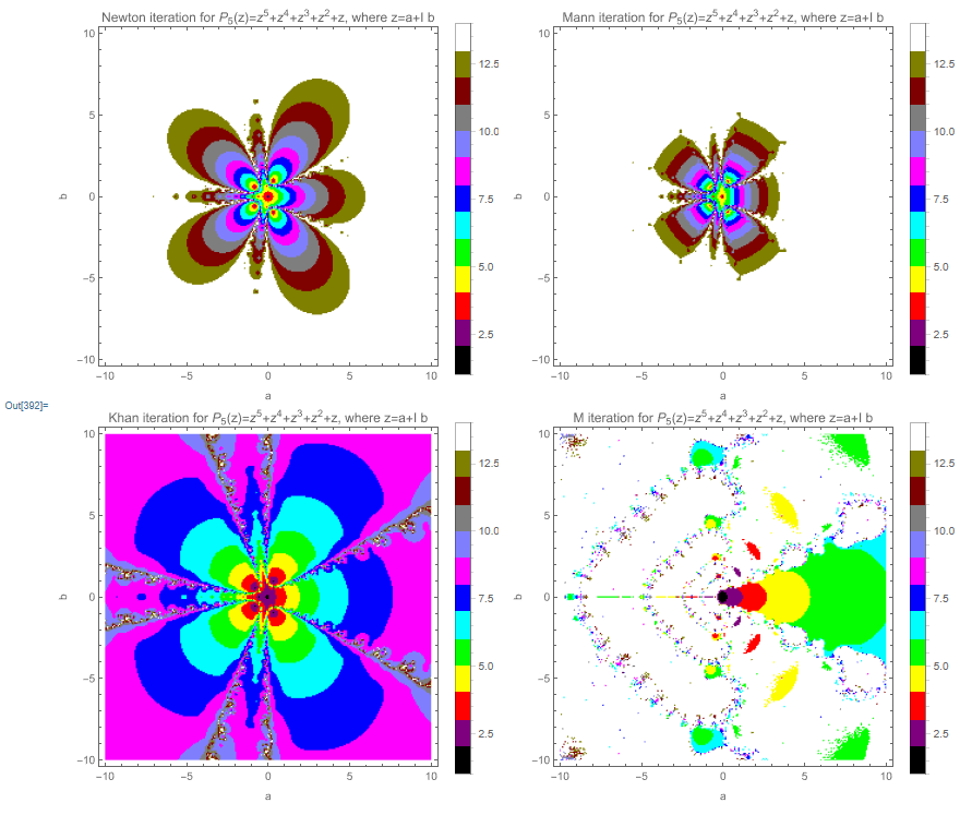
Similar results can be produced for P5 (following the reference the plot range is changed here):

m=250;
aRange=Subdivide [-10.,10.,m];
bRange=aRange;

P5newton=Quiet@ParallelTable[{a,b,Quiet@iteration[P5Tnewton,P5roots,13][a+I b]},{a,aRange},{b,bRange},DistributedContexts->All];
P5mann=Quiet@ParallelTable[{a,b,Quiet@iteration[P5Tmann,P5roots,13][a+I b]},{a,aRange},{b,bRange},DistributedContexts->All];
P5khan=Quiet@ParallelTable[{a,b,Quiet@iteration[P5Tkahn,P5roots,13][a+I b]},{a,aRange},{b,bRange},DistributedContexts->All];
P5M=Quiet@ParallelTable[{a,b,Quiet@iteration[P5TM,P5roots,13][a+I b]},{a,aRange},{b,bRange},DistributedContexts->All];

ClearAll[m,aRange,bRange];

colorFuntion=Function[{k},If[k<0||k>13,White,{RGBColor[0.001,0.001,0.001],RGBColor[0.001,0.001,0.001],RGBColor[0.494,0.001,0.494],RGBColor[0.994,0.007,0.001],RGBColor[0.992,0.993,0.001],RGBColor[0.012,0.995,0.002],RGBColor[0.001,0.993,0.992],RGBColor[0.013,0.006,0.995],RGBColor[0.991,0.001,0.994],RGBColor[0.497,0.5,0.995],RGBColor[0.496,0.495,0.494],RGBColor[0.499,0.003,0.002],RGBColor[0.5,0.5,0.001],RGBColor[1.,1.,1.]}[[Floor[k]+1]]]];

plot=ListDensityPlot[Flatten[#1,1],PlotLegends->Placed[BarLegend[{colorFuntion,{1,14}}],Right],InterpolationOrder->0,PlotRange->All,ColorFunction->colorFuntion,ColorFunctionScaling->False,FrameLabel->{"a","b"},PlotLabel->#2<>" iteration for Subscript[P, 5](z)=z^5+z^4+z^3+z^2+z, where z=a+I b",ImageSize->350]&;
Grid[{{plot[P5newton,"Newton"],plot[P5mann,"Mann"]},{plot[P5khan,"Khan"],plot[P5M,"M"]}}]
Clear[plot]

resulting in

EDIT: Following the first three comments on this answer I modified it to include M-iteration with fixed $\alpha_n=0.9$ and $T_\mathrm{Newton}$ as operator $T$. Compared to the original answer I changed the operators $T$ as well as the iteration routine to work with non-constant/functional $\alpha$: instead of the constant function 0.9& one could try out any function of n, e.g. 1.+#&. Concerning the M-iteration from the comments: I tried it only with $T=T_\mathrm{Newton}$ and constant $\alpha_n$ which seems to work rather poorly for $P_5(z)$. Other choices for $T$ and $\alpha_n$ might work better. To speed up the data generation I switched to using ParallelTable but most of the execution time is spent generating the plots.