LinearModelFit for ANCOVA Issues with Fitted Model & Plot with Bonferroni F-value corrections

Question

In attempting to modify the example for generating an ANCOVA model for my data (data3), which is for purposes of illustration the first 20 and the last 20 records of a larger dataset. Here, I seek to compare two rather than four groups given in the example, I have encountered several issues that I do not understand and that leave me wondering if my modifications are correct. Unlike the example that uses generated data for 4 treatments, I am comparing two measurements (standard length and head length) from two different species (treatments/groups). These data are in mm.

data3 = {{1, 220.5, 107.2}, {1, 150.8, 70.6}, {1, 74.52, 33.71}, {1, 76.3, 
        35.1}, {1, 74.59, 34.52}, {1, 95.77, 45.32}, {1, 74.52, 33.71}, {1, 
        96.66, 44.32}, {1, 104.1, 49.7}, {1, 89., 41.1}, {1, 79.1, 
        38.1}, {1, 76.46, 33.83}, {1, 228.5, 103.7}, {1, 170.2, 81.8}, {1, 
        218.5, 99.5}, {1, 238., 105.8}, {1, 243.9, 112.}, {1, 65.67, 
        27.39}, {1, 103.81, 45.63}, {1, 95.29, 41.8}, {2, 111.27, 
        51.77}, {2, 174.05, 82.05}, {2, 166.15, 80.3}, {2, 51.74, 
        23.37}, {2, 196.4, 89.91}, {2, 96.58, 43.05}, {2, 168.82, 
        72.47}, {2, 181.95, 83.14}, {2, 132.11, 61.34}, {2, 105.82, 
        46.6}, {2, 112.36, 54.53}, {2, 72.19, 31.}, {2, 62.14, 28.89}, {2, 
        64.81, 26.84}, {2, 47.11, 22.27}, {2, 95.45, 49.19}, {2, 208.49, 
        97.}, {2, 116.02, 53.84}, {2, 105., 51.6}, {2, 106.6, 48.3}}

Following the example, I then execute the following modification:

 lm = LinearModelFit[data3, {species, sl}, {species, sl}, 
  NominalVariables -> species];
  Grid[{{lm["ANOVATable"]}, {Show[ListPlot[Drop[
  GatherBy[Sort[data3], First], None, None, 1], 
  PlotRange -> {{0, Max[data2[[All, 2]]]}, {0, 
    Max[data2[[All, 3]]]}}], 
  Plot[Evaluate[Map[lm[#, t] &, groups3]], {t, 0, 250}]]}, {lm}}]

I get the ANOVATable, with some suspicious P-values, followed by the plot, which seems to be missing the calulated least square fit line for either species, and a fitted model that I do not understand that reads:

FittedModel[ -1.94155 + 0.463712 SL - 0.294817 DiscreteIndicator[species,1,(1,2)]

Why is the plot of the least-squares line of best fit missing? I have substituted 250 for the range of "t", since the highest possible value of SL is about 250, but this interpretation may be at odds with the example.

If I am interpreting the fitted model output correctly, the result can be interpreted as the HL (data3[[All,3]] = the y-intercept (HL= -1.94155) + the slope (0.463712 *SL) - the adjusted mean resulting from the variance attributable to being different species (0.294817) given equal slopes for the two species. However, I am confused by the meaning of DiscreteIndicator[species,1,(1,2)], which I suspect, simply reflects the fact that species in the first column of data3 is regarded as the dummy variable. Is this interpretation correct?

The very small P-values suggest that the adjusted means are not the same, even though from the plot (even of this small amount of data) the two species appear to be virtually identical with respect to these variables. Is my suspicion that the adjusted means are NOT significantly different justified?

Likewise, I am unsure how to obtain the critical Bonferroni or Sheffe F-Values to account for Type 1 Error for multiple comparisons from these results, when after a test for homogenetity of regression slopes prove that the slopes of different groups are statistically the same as they are for this contrast.

I have many such comparisons to make for other variables against SL and am eager to determine if my modification of the example code is correct so that these results can be extended for multiple comparisons (about 40) for which it seems prudent to use suitably corrected F-Values to compute the probability that the adjusted means are in fact different when the slopes are not.

Can anyone set me straight as to how to compute this ANCOVA properly and to extend it with a Bonferroni or Sheffe correction? Thanks.

Answer 1

Your model fit and ANOVA table are

lm = LinearModelFit[data3, {species, sl}, {species, sl}, NominalVariables -> species];
lm["ANOVATable"]

The P-value of 9.08206 x 10^-7 looks "suspicious" but that's because that P-value isn't what you think it is. Mathematica is using what is called (in SAS lingo) "Type I Sums of Squares" or "Sequential sum of squares". This is the sum of squares associated with species unadjusted for the covariate (sl = standard length). (And more generally sequential sums of squares are "adjusted for terms preceding it and unadjusted for terms following it".)

You can get an appropriate P-value for testing whether the intercepts for both species are identical by simply changing {species, sl}, {species, sl} to {sl, species}, {species, sl}.

lm = LinearModelFit[data3, {sl, species}, {species, sl}, NominalVariables -> species]
lm["ANOVATable"]

Does that sound crazy? Yes, it does. I love Mathematica but it has a long ways to go before I would use it for analysis of variance or analysis of covariance.

Addition

If you need to do a lot of multiple comparisons and want to use various adjustments (such as Tukey, Bonferroni, etc.), you should use R or SAS rather than Mathematica. But if you're just interested in all possible pairwise comparisons from a simple ANCOVA, here's one (convoluted) way to do it.

Create some data.

groups = {"control", "treatment 1", "treatment 2", "treatment 3"};

data = BlockRandom[SeedRandom[123];
   Block[{vals, times, rand}, vals = RandomChoice[groups, 100];
    times = RandomInteger[10, 100];
    rand = RandomReal[1, 100];
    Transpose[{vals, times, (vals /. 
         Thread[Rule[groups, {.16, .34, .57, 1.1}]]) - .05 times + rand}]]];

Fit the model and get estimates of parameters.

lm = LinearModelFit[data, {treatment, time}, {treatment, time}, 
  NominalVariables -> treatment, IncludeConstantBasis -> False]
estimates = lm["BestFitParameters"];
cov = lm["CovarianceMatrix"];

Now find all possible differences in the treatments (i.e., the intercepts of a simple linear model).

(* Number of treatments *)
t = Length[groups]; 

(* Degrees of freedom for error *)
df = lm["ANOVATableDegreesOfFreedom"][[Length[ lm["ANOVATableDegreesOfFreedom"]] - 1]]
(* 95 *)

(* Indices of all possible pairwise comparisons *)
comparisons = Select[Sort[#] & /@ Tuples[Range[t], {2}], #[[1]] < #[[2]] &] // DeleteDuplicates
(* {{1,2},{1,3},{1,4},{2,3},{2,4},{3,4}} *)

(* Differences and standard errors of differences *)
diffs = estimates[[#[[1]]]] - estimates[[#[[2]]]] & /@ comparisons
(* {-0.070739, -0.425142, -0.814842, -0.354403, -0.744103, -0.389699} *)

seDiffs = Sqrt[cov[[#[[1]], #[[1]]]] + cov[[#[[2]], #[[2]]]] - 
     2 cov[[#[[1]], #[[2]]]]] & /@ comparisons
(* {0.0883031, 0.089601, 0.0895971, 0.0828474, 0.0879348, 0.0891328} *)

Now put together the pieces to determine the Bonferroni adjusted P-values and confidence limits for the pairwise differences:

tValues = (estimates[[#[[1]]]] - estimates[[#[[2]]]])/
    Sqrt[cov[[#[[1]], #[[1]]]] + cov[[#[[2]], #[[2]]]] - 
      2 cov[[#[[1]], #[[2]]]]] & /@ comparisons
(* {-0.801093, -4.74484, -9.09451, -4.27779, -8.46198, -4.37212} *)

Pvalues = 2*CDF[StudentTDistribution[df], -Abs[#]] & /@ tValues
(* {0.425077, 7.34947*10^-6, 1.42412*10^-14, 0.0000449881,  3.17124*10^-13, 0.0000314736} *)

α = 0.05/Length[comparisons]
(* 0.00833333 *)

confLimits = Transpose[{diffs - InverseCDF[StudentTDistribution[95], 1 - α/2] seDiffs,
   diffs + InverseCDF[StudentTDistribution[95], 1 - α/2] seDiffs}]
(* {{-0.308683, 0.167205}, {-0.666584, -0.183701}, {-1.05627, 0.573411}, 
    {-0.577646, -0.131161}, {-0.981054, -0.507151}, {-0.629879, -0.14952}} *)

Second addition

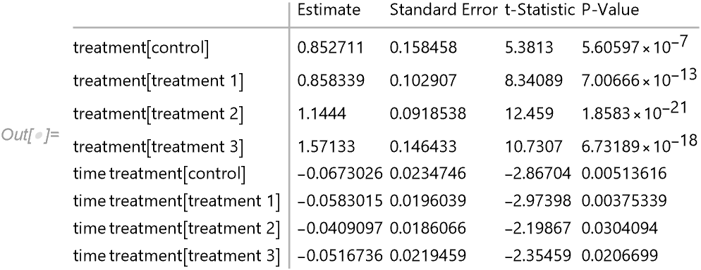
With the above data one can also fit separate intercepts and separate slopes with LinearModelFit:

lm = LinearModelFit[data, {treatment, treatment*time}, {treatment, time}, 
  NominalVariables -> treatment, IncludeConstantBasis -> False];
lm["ParameterTable"]

Third addition

If you want to get a test for equal slopes:

lm = LinearModelFit[data, {treatment, x, treatment*x}, {treatment, x},
    NominalVariables -> treatment];
lm["ANOVATable"]

So the P-value for testing equal slopes is 0.832571. (I would still suggest using R or SAS for anything beyond a basic ANOVA as with Mathematica while you can get all of the right tests, there is a lot of handwork which can easily result in coding errors.)