Added approach to get an appropriate test for equal slopes.
Source Link
JimB
  • 42.9k
  • 3
  • 51
  • 108

Third addition

If you want to get a test for equal slopes:

lm = LinearModelFit[data, {treatment, x, treatment*x}, {treatment, x},
    NominalVariables -> treatment];
lm["ANOVATable"]

ANOVA table with test for equal slopes

So the P-value for testing equal slopes is 0.832571. (I would still suggest using R or SAS for anything beyond a basic ANOVA as with Mathematica while you can get all of the right tests, there is a lot of handwork which can easily result in coding errors.)

Added example of fitting separate slopes in addition to separate intercepts.
Source Link
JimB
  • 42.9k
  • 3
  • 51
  • 108

Second addition

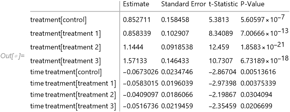
With the above data one can also fit separate intercepts and separate slopes with LinearModelFit:

lm = LinearModelFit[data, {treatment, treatment*time}, {treatment, time}, 
  NominalVariables -> treatment, IncludeConstantBasis -> False];
lm["ParameterTable"]

Parameter table

Second addition

With the above data one can also fit separate intercepts and separate slopes with LinearModelFit:

lm = LinearModelFit[data, {treatment, treatment*time}, {treatment, time}, 
  NominalVariables -> treatment, IncludeConstantBasis -> False];
lm["ParameterTable"]

Parameter table

Added blurb on constructing Bonferroni adjustments for a simple ANCOVA
Source Link
JimB
  • 42.9k
  • 3
  • 51
  • 108

Addition

If you need to do a lot of multiple comparisons and want to use various adjustments (such as Tukey, Bonferroni, etc.), you should use R or SAS rather than Mathematica. But if you're just interested in all possible pairwise comparisons from a simple ANCOVA, here's one (convoluted) way to do it.

Create some data.

groups = {"control", "treatment 1", "treatment 2", "treatment 3"};

data = BlockRandom[SeedRandom[123];
   Block[{vals, times, rand}, vals = RandomChoice[groups, 100];
    times = RandomInteger[10, 100];
    rand = RandomReal[1, 100];
    Transpose[{vals, times, (vals /. 
         Thread[Rule[groups, {.16, .34, .57, 1.1}]]) - .05 times + rand}]]];

Fit the model and get estimates of parameters.

lm = LinearModelFit[data, {treatment, time}, {treatment, time}, 
  NominalVariables -> treatment, IncludeConstantBasis -> False]
estimates = lm["BestFitParameters"];
cov = lm["CovarianceMatrix"];

Now find all possible differences in the treatments (i.e., the intercepts of a simple linear model).

(* Number of treatments *)
t = Length[groups]; 

(* Degrees of freedom for error *)
df = lm["ANOVATableDegreesOfFreedom"][[Length[ lm["ANOVATableDegreesOfFreedom"]] - 1]]
(* 95 *)

(* Indices of all possible pairwise comparisons *)
comparisons = Select[Sort[#] & /@ Tuples[Range[t], {2}], #[[1]] < #[[2]] &] // DeleteDuplicates
(* {{1,2},{1,3},{1,4},{2,3},{2,4},{3,4}} *)

(* Differences and standard errors of differences *)
diffs = estimates[[#[[1]]]] - estimates[[#[[2]]]] & /@ comparisons
(* {-0.070739, -0.425142, -0.814842, -0.354403, -0.744103, -0.389699} *)

seDiffs = Sqrt[cov[[#[[1]], #[[1]]]] + cov[[#[[2]], #[[2]]]] - 
     2 cov[[#[[1]], #[[2]]]]] & /@ comparisons
(* {0.0883031, 0.089601, 0.0895971, 0.0828474, 0.0879348, 0.0891328} *)

Now put together the pieces to determine the Bonferroni adjusted P-values and confidence limits for the pairwise differences:

tValues = (estimates[[#[[1]]]] - estimates[[#[[2]]]])/
    Sqrt[cov[[#[[1]], #[[1]]]] + cov[[#[[2]], #[[2]]]] - 
      2 cov[[#[[1]], #[[2]]]]] & /@ comparisons
(* {-0.801093, -4.74484, -9.09451, -4.27779, -8.46198, -4.37212} *)

Pvalues = 2*CDF[StudentTDistribution[df], -Abs[#]] & /@ tValues
(* {0.425077, 7.34947*10^-6, 1.42412*10^-14, 0.0000449881,  3.17124*10^-13, 0.0000314736} *)

α = 0.05/Length[comparisons]
(* 0.00833333 *)

confLimits = Transpose[{diffs - InverseCDF[StudentTDistribution[95], 1 - α/2] seDiffs,
   diffs + InverseCDF[StudentTDistribution[95], 1 - α/2] seDiffs}]
(* {{-0.308683, 0.167205}, {-0.666584, -0.183701}, {-1.05627, 0.573411}, 
    {-0.577646, -0.131161}, {-0.981054, -0.507151}, {-0.629879, -0.14952}} *)
Source Link
JimB
  • 42.9k
  • 3
  • 51
  • 108
Loading