Making LinearModelFit account for Log on the x-axis

Question

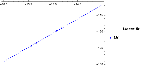
I have the following code that I wish to run, which consists of 6 data points that I want to fit using LinearModelFit

Clear["Global`*"]

ϕ0 = 2.068*10^-15;(*femto-Tm^2*)
zchar = 50;
LLl1 = 500*10^-12(*H*);
LLl2 = 900*10^-12(*H*);
LLl3 = 1000*10^-12(*H*);
LLl4 = 1500*10^-12(*H*);
LLl5 = 1670*10^-12(*H*);
LLl6 = 2000*10^-12(*H*);
I01 = ϕ0/(2 π*LLl1);
I02 = ϕ0/(2 π*LLl2);
I03 = ϕ0/(2 π*LLl3);
I04 = ϕ0/(2 π*LLl4);
I05 = ϕ0/(2 π*LLl5);
I06 = ϕ0/(2 π*LLl6);

Il1 = 0.0257399*Sqrt[2]*(28.3346/26.26)*(0.5*I01)(*As/Ap*Sqrt[2]*(ωs/ωp)(0.5*I0) for 20.0227dB \gain*);
Il2 = 0.0257399*Sqrt[2]*(15.5602/14.43)*(0.5*I02)(*As/Ap*Sqrt[2]*(ωs/ωp)(0.5*I0) for 20.004dB \gain*);
Il3 = 0.0261556*Sqrt[2]*(13.985/12.97)*(0.5*I03)(*As/Ap*Sqrt[2]*(ωs/ωp)(0.5*I0) for 20.0038dB \gain*);
Il4 = 0.0257399*Sqrt[2]*(9.28253/8.61)*(0.5*I04)(*As/Ap*Sqrt[2]*(ωs/ωp)(0.5*I0) for 20.0358dB \gain*);
Il5 = 0.0257399*Sqrt[2]*(8.33335/7.73)*(0.5*I05)(*As/Ap*Sqrt[2]*(ωs/ωp)(0.5*I0) for 20.0318dB \gain*);
Il6 = 0.0261566*Sqrt[2]*(6.95093/6.448)*(0.5*I06)(*As/Ap*Sqrt[2]*(ωs/ωp)(0.5*I0) for 20.006dB \gain*);

pl1 = (Il1^2*zchar)/2*1000(*in milliWatts*);
pl2 = (Il2^2*zchar)/2*1000(*in milliWatts*);
pl3 = (Il3^2*zchar)/2*1000(*in milliWatts*);
pl4 = (Il4^2*zchar)/2*1000(*in milliWatts*);
pl5 = (Il5^2*zchar)/2*1000(*in milliWatts*);
pl6 = (Il6^2*zchar)/2*1000(*in milliWatts*);

pointsLHTL = {{I01, 10 Log10[pl1]}, {I02, 10 Log10[pl2]}, {I03, 
10 Log10[pl3]}, {I04, 10 Log10[pl4]}, {I05, 10 Log10[pl5]}, {I06, 10 Log10[pl6]}};


LHdynamicrange = 
ListLogLinearPlot[Evaluate@pointsLHTL, 
PlotRange -> {Automatic, Automatic}, 
LabelStyle -> Directive[Black, 12], PlotLegends -> {"LH"}, 
Joined -> False, ImageSize -> Large, 
PlotStyle -> Directive[Blue]]

Lm = LinearModelFit[Log@pointsLHTL, x, x]
Lmplot = Plot[Lm[x], {x, -16, -14}, 
PlotStyle -> Directive[Blue, Dashed], PlotLegends -> {"Linear fit"}]

Show[Lmplot, LHdynamicrange]

where pointsLHTL represent my data points (with the y-values under Log10 and multiplied by 10). LHdyanmicrange is a ListLogLinearPlot of pointsLHTL as I want the x-axis to be under Log scale as well (natural in this case).

However, my fitting curve Lm and its plot Lmplot does not account for the Log values as shown in LHdynamicrange. How can I adjust my Lmplot or Lm so that it incorporates the Log scale similar to LHdynamicrange when I Show both of them on the same plot?

Thanks

Answer 1

The problem is that you are evaluating Log on all elements of pointsLHTL, not just the x values. The y values are negative so the Log is imaginary.

Lm = LinearModelFit[pointsLHTL /. {x_, y_} :> {Log@x, y}, x, x]

Lmplot = 
 Plot[Lm[x], {x, -16, -14}, PlotStyle -> Directive[Blue, Dashed], 
  PlotLegends -> {"Linear fit"}]

Show[Lmplot, LHdynamicrange]