How can I speed up RandomVariate in the following case?

Question

I would like to generate random values of some parameter with the weight being the Poisson distribution. An important point is that each time I generate the random number I need to consider the distribution with different 1st momentum, that I parametrize by $\gamma$:

$$ f_{\gamma}(x) = \frac{1}{2\gamma}\exp\left[-\frac{x}{2\gamma}\right] $$

I make a grid with 100000 values of $\gamma$, but then find that the procedure of generating the random values is extremely slow, requiring $\mathcal{O}(10^{3})$ s on my machine. How can I speed up the code?

My code is given below:

dist[gamma_] :=
  ProbabilityDistribution[
   Exp[-(x/(2*gamma))] 1/(2*gamma), {x, 0, Infinity}];
Tabgamma = Table[RandomReal[{1, 100}], {i, 1, 10^5, 1}];
TabRV = Table[RandomVariate[dist[Tabgamma[[i]]]], {i, 1, 10, 1}] //
  AbsoluteTiming

(*{0.111845, {38.0185, 162.312, 396.125, 53.1418, 81.3972, 4.29874, 37.5393, 27.0455, 15.5522, 28.2158}}*)

Answer 1

@BobHanlon beat me to it. But on second thought, I think this produces the TabRV table with all 100,000 values of $\gamma$ about 250 times faster.

I don't know what the Poisson distribution or weighting has to do with what you want to do. However, one can speed up your code greatly by first determining the inverse cdf of your random variable:

dist[gamma_] := ProbabilityDistribution[Exp[-(x/(2*gamma))] 1/(2*gamma), {x, 0, Infinity}];
InverseCDF[dist[γ], u]

Then you can take random samples from uniform distribution with the 100,000 values of $\gamma$ and obtain the samples for TabRV:

SeedRandom[12345];
Tabgamma = Table[RandomReal[{1, 100}], {i, 1, 10^5, 1}];
u = RandomReal[{0, 1}, Length[Tabgamma]];
AbsoluteTiming[TabRV = -2 Tabgamma Log[1 - u];]
(* {0.0015765, Null} *)

Answer 2

Clear["Global`*"]

dist[gamma_] := 
  ProbabilityDistribution[Exp[-(x/(2*gamma))] 1/(2*gamma), 
   {x, 0, Infinity}];

The distribution dist is equivalent to the built-in ExponentialDistribution. It is far more efficient to use the built-in distributions.

dist2[gamma_] = ExponentialDistribution[1/(2 gamma)];

PDF[dist2[gamma], x]

(* Piecewise[{{1/(E^(x/(2*gamma))*(2*gamma)), x >= 0}}, 0] *)

Tabgamma = Table[RandomReal[{1, 100}], {i, 1, 10^5}];

SeedRandom[1234];

TabRV = Table[RandomVariate[dist[Tabgamma[[i]]]], {i, 1, 10}] // 
  RepeatedTiming

(* {0.122387, {157.332, 33.144, 8.66059, 3.10988, 73.2489, 26.4499, 279.908, 
  167.704, 167.158, 9.95176}} *)

TabRV2 = Table[RandomVariate[dist2[Tabgamma[[i]]]], {i, 1, 10}] // 
  RepeatedTiming

(* {0.0000282663, {167.878, 31.4419, 9.73242, 2.82922, 187.9, 208.963, 5.14213, 
  134.806, 168.164, 173.493}} *)

EDIT: For an analytical approach, use ParameterMixtureDistribution

dist3 = ParameterMixtureDistribution[
   ExponentialDistribution[1/(2 gamma)],
   gamma \[Distributed] UniformDistribution[{1, 100}]];

PDF[dist3, x]

Integrate[PDF[dist3, x], {x, 0, Infinity}]

(* 1 *)

cdf[x_] = CDF[dist3, x]

Limit[cdf[x], x -> #] & /@ {0, Infinity}

(* {0, 1} *)

Moment[dist3, r]

(* (2^r (-1 + 100^(1 + r)) r!)/(99 (1 + r)) *)

#[dist3] & /@ {Mean, Variance}

(* {101, 16735} *)

AbsoluteTiming[TabRV3 = RandomVariate[dist3, 10^5];]

(* {0.580082, Null} *)

This is much slower than the other proposed approaches, but is still much faster than the original.

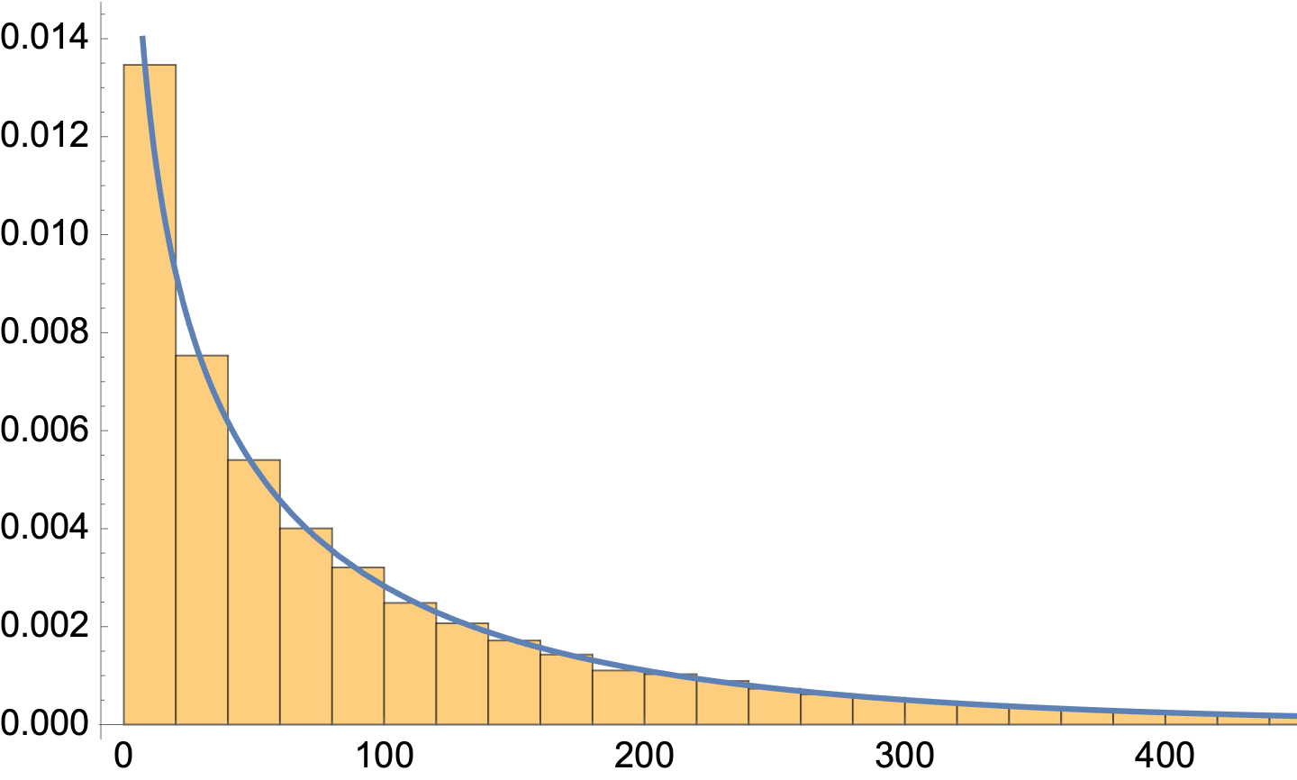
Show[
 Histogram[TabRV3, Automatic, "PDF"],
 Plot[Tooltip[PDF[dist3, x]], {x, 0, 450},
  PlotRange -> {0, 0.014}]]