Let's start by creating some example datasets:
signal = Table[Sin[x], {x, Subdivide[0, 2 Pi, 100]}];
noise = {
   RandomVariate[NormalDistribution[0.2, 0.1], 101],
   RandomVariate[NormalDistribution[0.1, 0.2], 101],
   RandomVariate[NormalDistribution[0.4, 0.3], 101],
   RandomVariate[NormalDistribution[-0.1, 0.3], 101],
   RandomVariate[NormalDistribution[-0.2, 0.25], 101]
   };
data = signal + # & /@ noise;

Dimensions[data]
{5, 101}
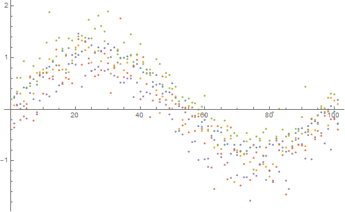
ListPlot[data, ImageSize -> 500]
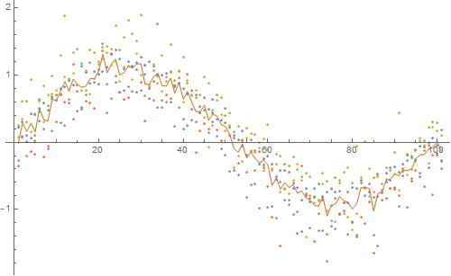
Now, for each point along the x-axis, compute the mean and standard deviation:
{mean, std} = Transpose[
   {Mean[#], StandardDeviation[#]} & /@ Transpose[data]
   ];

ListPlot[
 Append[data, mean],
 Joined -> {False, False, False, False, False, True},
 ImageSize -> 500
 ]
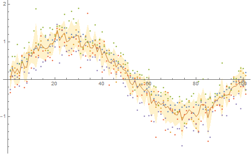
Now let us plot the standard deviation as a shaded area:
upper = mean + std;
lower = mean - std;
ListPlot[
 Join[data, {mean, upper, lower}],
 Joined -> {False, False, False, False, False, True, True, True},
 ImageSize -> 500,
 PlotStyle -> {Automatic, Automatic, Automatic, Automatic, Automatic, Automatic, None, None},
 Filling -> {8 -> {7}}
 ]
You may find further inspiration in the post Plot confidence interval around curve.
Please let me know if this is not what you were looking for.


Interpolateand then calculate data for common values of the independent variable. With these values you may get the mean and STD. $\endgroup$