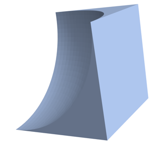
This is not a direct answer to your question, but an alternate approach. You could create a list of primitives and a build function that contains the Computational Solid Geometry (CSG).
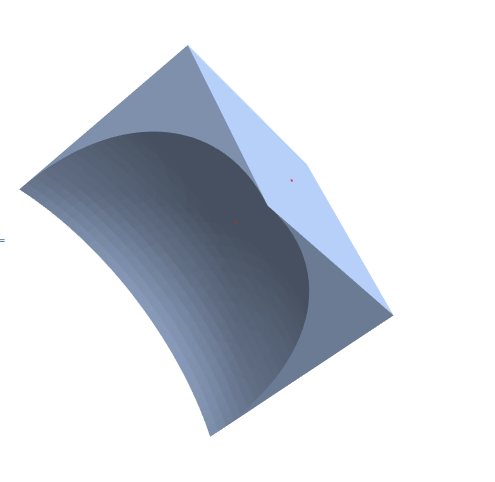
square = Cuboid[];
ball = Ball[{0, 0, 1}, 1];
buildList = {square, ball};
(* Constraints *)
buildFn = ¬ #2 ∧ #1 &;
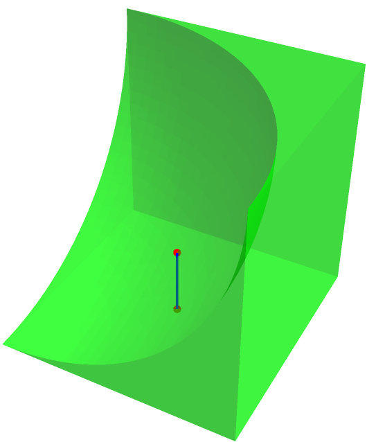
reg = Region[
   Style[BooleanRegion[buildFn, buildList], Opacity[0.5], Green]];
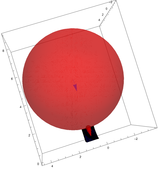
direction = {0, 0, -1};
point = {0.5, 0.5, 5};
line = HalfLine[{point, point + direction}];
rint = Region[RegionIntersection[reg, line],
  BaseStyle -> {Blue, Thick}];
intpoints = Point[Transpose@RegionBounds@rint];
Show[reg, rint, Graphics3D[{PointSize[Large], Red, intpoints}]]

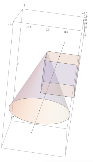
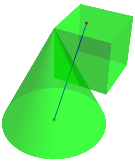
Here is how it would look for the initial case:
shape1 = Cone[];
shape2 = Cuboid[];
buildList = {shape1, shape2};
(* Constraints *)
buildFn = #2 || #1 &;
reg = Region[
   Style[BooleanRegion[buildFn, buildList], Opacity[0.5], Green]];
direction = {-0.2, -0.2, -1};
point = {0.5, 0.5, 1.5};
line = HalfLine[{point, point + direction}];
rint = Region[RegionIntersection[reg, line],
  BaseStyle -> {Blue, Thick}]; intpoints =
 Point[Transpose@RegionBounds@rint];
Show[reg, rint, Graphics3D[{PointSize[Large], Red, intpoints}],
 PlotRange -> All]

Update to Increase Speed
@Tomi mentioned in the comments that speed is a concern. As addressed in my answer to the MSE question Why is Ray Tracing Slow? I created a solver that that used the fast region functions RegionDistanceand RegionNormal to solve a 1000 multiple bounce ray traces in 3D geometry including geometry produced by a commercial CAD package. I will adapt that approach to look at the bouncing of single ray.
Set up the Geometry
The OpenCascadeLink does a pretty good job at constructing geometry that snaps to features while keeping the triangle count down. The following workflow will create the the initial Box-Cone geometry.
Needs["OpenCascadeLink`"]
Needs["NDSolve`FEM`"]
pp = Polygon[{{0, 0, 0}, {0, 0, 1}, {1, 0, 1}}];
shape = OpenCascadeShape[pp];
axis = {{0, 0, 0}, {0, 0, 1}};
sweep = OpenCascadeShapeRotationalSweep[shape, axis];
bmesh = OpenCascadeShapeSurfaceMeshToBoundaryMesh[sweep];
Show[Graphics3D[{{Red, pp}, {Blue, Thick, Arrow[axis]}}],
 bmesh["Wireframe"], Boxed -> False]
cu = OpenCascadeShape[Cuboid[{0, 0, 0}, {1, 1, 1}]];
union = OpenCascadeShapeUnion[cu, sweep];
bmesh = OpenCascadeShapeSurfaceMeshToBoundaryMesh[union];
groups = bmesh["BoundaryElementMarkerUnion"];
temp = Most[Range[0, 1, 1/(Length[groups])]];
colors = ColorData["BrightBands"][#] & /@ temp;
bmesh["Wireframe"["MeshElementStyle" -> FaceForm /@ colors]]
mrd = MeshRegion[bmesh, PlotTheme -> "Lines"]
Solve a Single Ray Trace
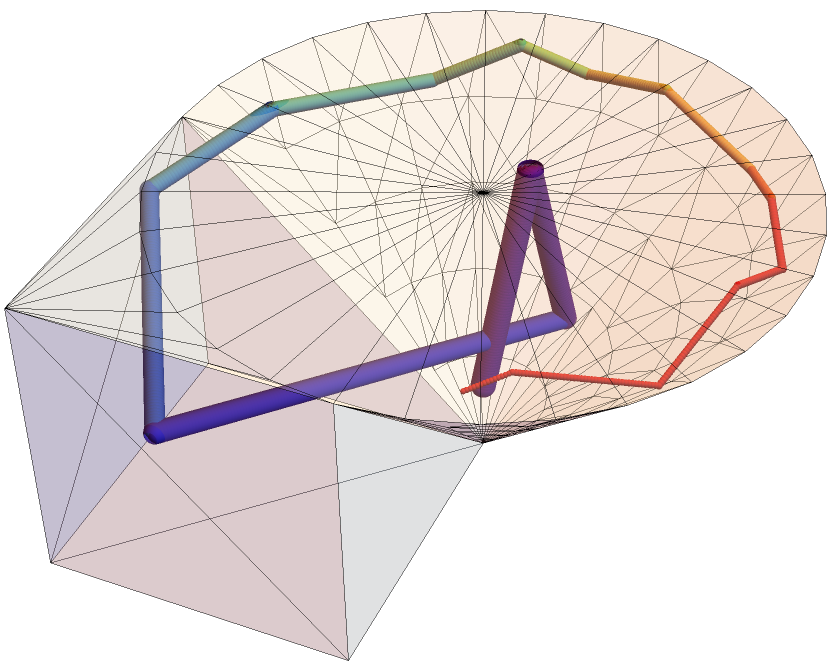
The following workflow solves for a single ray trace. Each bounce will cause the ray to attenuate the representative sphere size by 10%. This solves and plots quickly.
(* Set up Region Operators on Differenced Geometry *)
rdf = RegionDistance[mrd];
rnf = RegionNearest[mrd];
(* Setup and run simulation *)
(* Time Increment *)
dt = 0.01;
(* Collision Margin *)
margin = (1 + dt) dt;
(* Conditional Particle Advancer *)
advance[r_, x_, v_, c_] :=
 Block[{xnew = x + dt v}, {rdf[xnew], xnew, v, c}] /; r > margin
advance[r_, x_, v_, c_] :=
 Block[{xnew = x , vnew = v, normal = Normalize[x - rnf[x]]},
   vnew = Normalize[v - 2 v.normal normal];
   xnew += dt vnew;
   {rdf[xnew], xnew, vnew, c + 1}] /; r <= margin
(* Starting Point for Emission *)
sp = {0, 0, 0.25};
nparticles = 1;
ntimesteps = 800;
tabres = Table[
   NestList[
    advance @@ # &, {rdf[sp],
     sp, { Cos[2 Pi #[[1]]] Sin[Pi #[[2]]],
        Sin[ Pi #[[2]]] Sin[2 Pi #[[1]]], Cos[ Pi #[[2]]]} &@
      First@RandomReal[1, {1, 2}], 0}, ntimesteps], {i, 1,
    nparticles}];
epilog[i_] := {ColorData["Rainbow", (#4 - 1)/10],
    Sphere[#2, 0.04 0.9^#4]} & @@@ tabres[[i]]
Graphics3D[{White, EdgeForm[Thin], Opacity[0.25], mrd, Opacity[1]}~
  Join~epilog[1], Boxed -> False, PlotRange -> RegionBounds[mrd],
 ViewPoint -> {-1.7742436871276688`, 1.5459832360779067`,
   2.431459473742817`},
 ViewVertical -> {0.052110700162003136`, -0.06948693625348555`,
   0.9962208794332359`}]

A More Complex Case
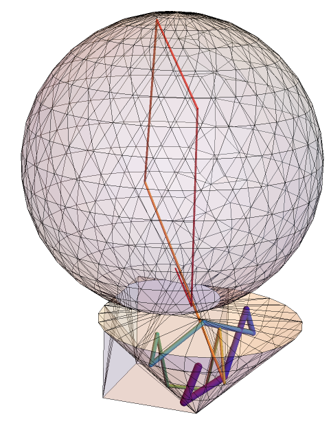
The following produces a shape with concavity that could find rays that intersect but would be blocked by an intervening surface. Because the solver use a fine time increment, these intersections are not found because the collision of the intervening surface is detected.
pp = Polygon[{{0, 0, 0}, {0, 0, 1}, {1, 0, 1}}];
shape = OpenCascadeShape[pp];
axis = {{0, 0, 0}, {0, 0, 1}};
sweep = OpenCascadeShapeRotationalSweep[shape, axis];
bmesh = OpenCascadeShapeSurfaceMeshToBoundaryMesh[sweep];
Show[Graphics3D[{{Red, pp}, {Blue, Thick, Arrow[axis]}}],
 bmesh["Wireframe"], Boxed -> False]
cu = OpenCascadeShape[Cuboid[{0, 0, 0}, {1, 1, 1}]];
ball = OpenCascadeShape[Ball[{1/2, 1/2, 2.4}, 1.5]];
union = OpenCascadeShapeUnion[cu, sweep, ball];
bmesh = OpenCascadeShapeSurfaceMeshToBoundaryMesh[union];
groups = bmesh["BoundaryElementMarkerUnion"];
temp = Most[Range[0, 1, 1/(Length[groups])]];
colors = ColorData["BrightBands"][#] & /@ temp;
bmesh["Wireframe"["MeshElementStyle" -> FaceForm /@ colors]]
mrd = MeshRegion[bmesh, PlotTheme -> "Lines"]
(* Set up Region Operators on Differenced Geometry *)
rdf = RegionDistance[mrd];
rnf = RegionNearest[mrd];
(* Setup and run simulation *)
(* Time Increment *)
dt = 0.01;
(* Collision Margin *)
margin = (1 + dt) dt;
(* Conditional Particle Advancer *)
advance[r_, x_, v_, c_] :=
 Block[{xnew = x + dt v}, {rdf[xnew], xnew, v, c}] /; r > margin
advance[r_, x_, v_, c_] :=
 Block[{xnew = x , vnew = v, normal = Normalize[x - rnf[x]]},
   vnew = Normalize[v - 2 v.normal normal];
   xnew += dt vnew;
   {rdf[xnew], xnew, vnew, c + 1}] /; r <= margin
(* Starting Point for Emission *)
sp = {0, 0, 0.5};
nparticles = 1;
ntimesteps = 1600;
(*tabres= Table[NestList[advance@@#&,{rdf[sp],sp,{ Cos[2 Pi #[[1]]] \
Sin[Pi #[[2]]],Sin[ Pi #[[2]]] Sin[2 Pi #[[1]]], Cos[ Pi \
#[[2]]]}&@First@RandomReal[1,{1,2}],0},ntimesteps],{i,1,nparticles}];*)


tabres = Table[
   NestList[
    advance @@ # &, {rdf[sp],
     sp, { Cos[2 Pi #[[1]]] Sin[Pi #[[2]]],
        Sin[ Pi #[[2]]] Sin[2 Pi #[[1]]], Cos[ Pi #[[2]]]} &@
      First@{{0.3788624698388783`, 0.8749177935911279`}}, 0},
    ntimesteps], {i, 1, nparticles}];
epilog[i_] := {ColorData["Rainbow", (#4 - 1)/12],
    Sphere[#2, 0.04 0.9^#4]} & @@@ tabres[[i]]
Graphics3D[{White, EdgeForm[Thin], Opacity[0.25], mrd, Opacity[1]}~
  Join~epilog[1], Boxed -> False, PlotRange -> RegionBounds[mrd],
 ViewPoint -> {-3.102894731729034`, -1.0062787100553268`,
   0.8996929706836663`},
 ViewVertical -> {-0.34334064946409365`, -0.07403103185215265`,
   0.93628874005217`}]
