4
$\begingroup$

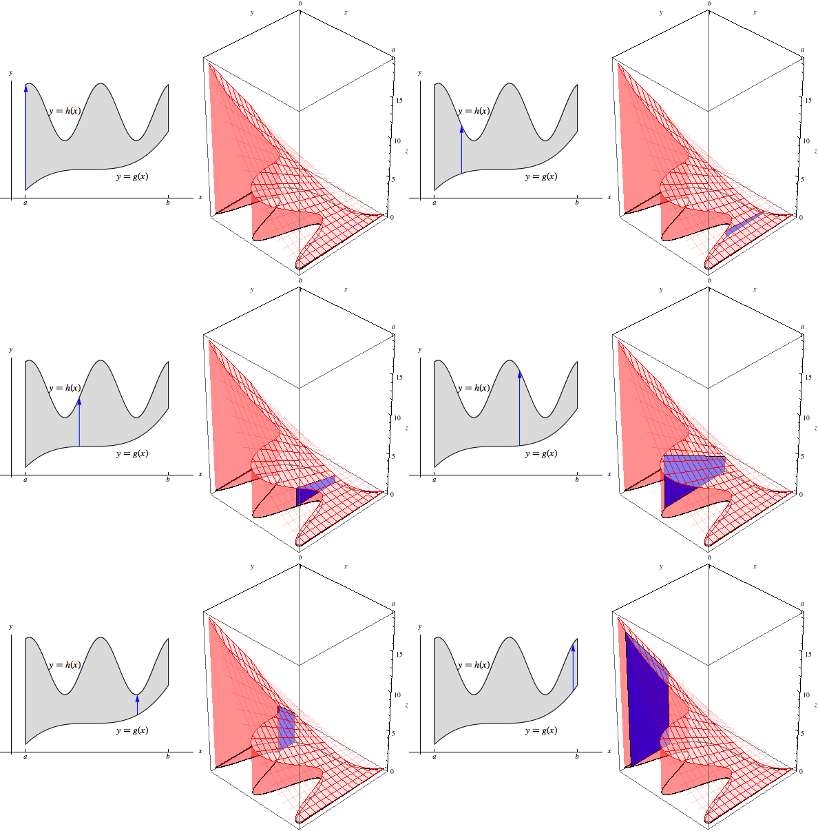
This question is related to a previous question Create a slider to illustrate Fubini theorem.

Thank to the help of @kglr, now I can create sliders to control the slice.

 ClearAll[a, B1, B2, B3, B4];

B4[a_?NumericQ] := 
 ParametricPlot3D[{a, y, z}, {y, 
   3 + (-8 + a)* (1/13 + (0.01 + 0.0022*(-4 + a))*(5 + a)), 
   4.8 + Sin[a]}, {z, 0, 0.01*(a + 5)^2}, PlotPoints -> 100, 
  Mesh -> 20, 
  PlotStyle -> 
   Directive[Blue, Opacity[0.4], Thickness[0.06], 
    Specularity[White, 30]]];(*The blue plane*)

B1 = 
 ParametricPlot3D[{x, y, 0.01*(x + 5)^2}, {x, -5, 5}, {y, 
   3 + (-8 + x) (1/13 + (0.01 + 0.0022*(-4 + x))*(5 + x)), 
   4.8 + Sin[x]}, Mesh -> 20, PlotStyle -> Opacity[0], 
  MeshStyle -> Opacity[.8], 
  PlotStyle -> 
   Directive[Blue, Opacity[0.3], Specularity[White, 30]]];

B2 = ParametricPlot3D[{x, 
    3 + (-8 + x) (1/13 + (0.01 + 0.0022*(-4 + x))*(5 + x)), 
    z}, {x, -5, 5}, {z, 0, 0.01*(x + 5)^2}, PlotPoints -> 100, 
   Mesh -> 20, MeshStyle -> Opacity[.1], 
   PlotStyle -> 
    Directive[Green, Opacity[0.3], Specularity[White, 30]]];

B3 = ParametricPlot3D[{x, 4.8 + Sin[x], z}, {x, -5, 5}, {z, 0, 
    0.01*(x + 5)^2}, PlotPoints -> 100, Mesh -> 20, 
   MeshStyle -> Opacity[.1], 
   PlotStyle -> 
    Directive[Red, Opacity[0.4], Specularity[White, 30]]];

t1 = Manipulate[
   Show[B1, B2, B3, B4[a], AxesStyle -> Thick, Boxed -> False, 
    AxesOrigin -> {0, 0, 0}, AxesLabel -> {x, y, z}, 
    BoxRatios -> {1, 1, 1.3}], {{a, 1}, -5, 5}];

t2 = Plot[{4.8 + Sin[x], 
    3 + (-8 + x) (1/13 + (0.01 + 0.0022*(-4 + x))*(5 + x))}, {x, -5, 
    5}, PlotRange -> {1.7, 6}];

t3[a_?NumericQ] := 
  Plot[100* Sign[x - a], {x, -5, 5}, ExclusionsStyle -> Blue, 
   PlotRange -> {3 + (-8 + a) (1/
         13 + (0.01 + 0.0022*(-4 + a))*(5 + a)), 4.8 + Sin[a]}];

t4 = Manipulate[Show[t2, t3[a]], {{a, 1}, -5, 5}];


 Grid[{{t1, t4}}, ItemSize -> {{30, 30}}, Frame -> All, 
     FrameStyle -> Red]

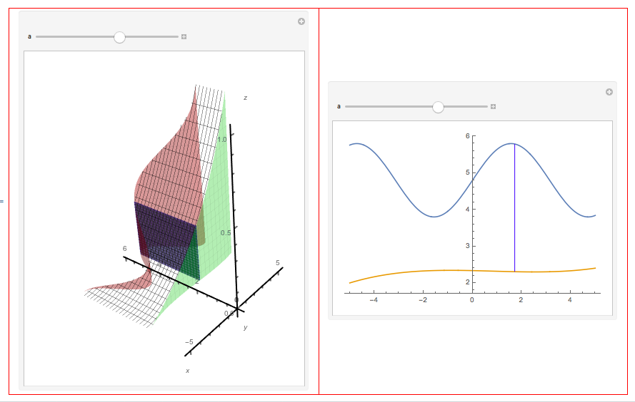
enter image description here

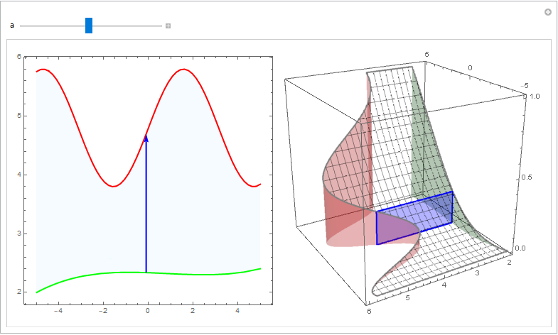
My question: How can we create only one slider for $a$ to control two graphs? The parameter $a$ for the picture on the left is used for the plane $x=a$ (the blue plane), while the same $a$ is for the line $x=a$ on the right hand side picture. That is, we will have the following illustration.

enter image description here

Thank for any hint.

$\endgroup$

3 Answers 3

1
$\begingroup$

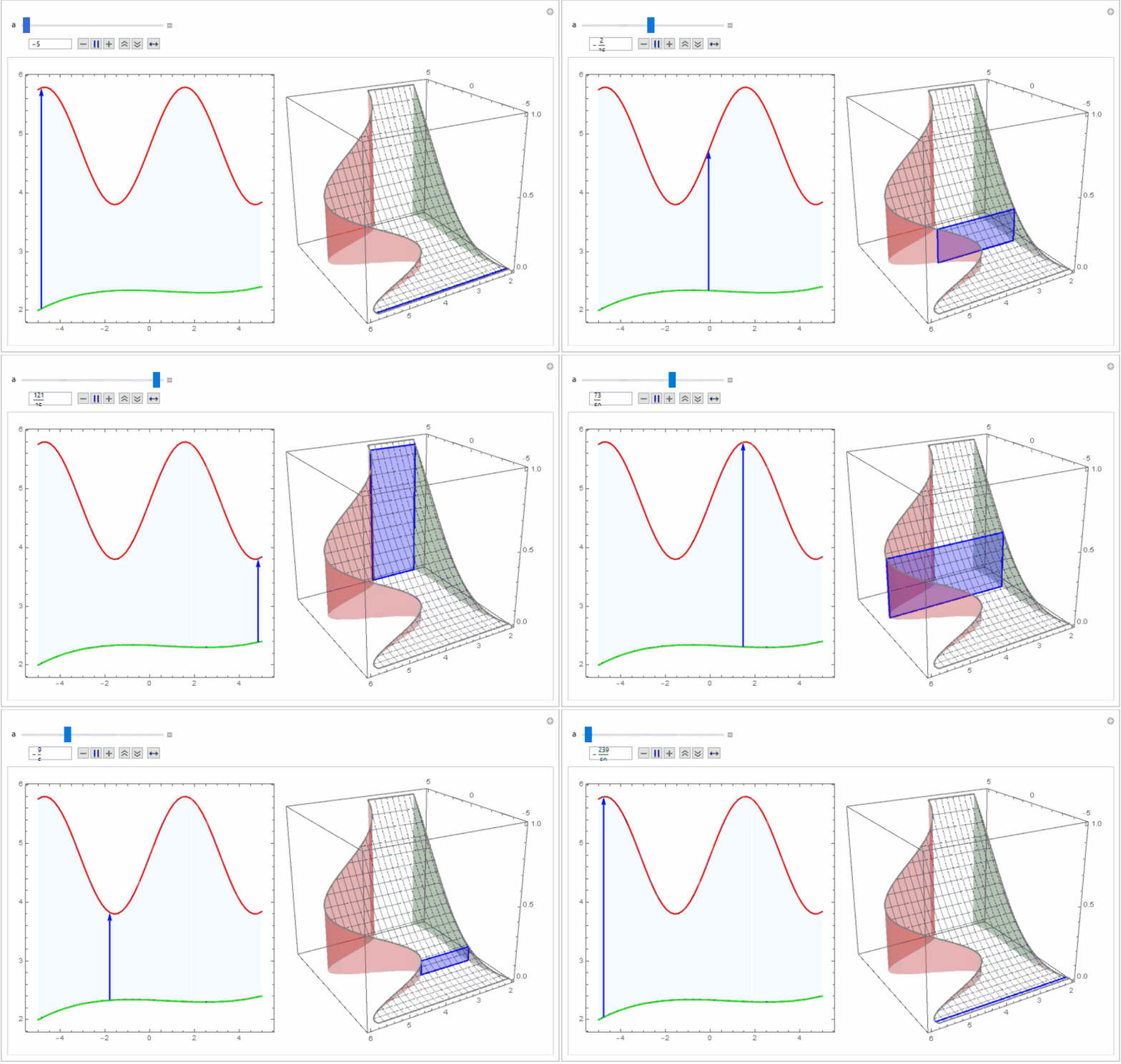
enter image description here

Code

ClearAll[f1, f2, f3]
f1[x_] := 4.8 + Sin[x]
f2[x_] := 3 + (-8 + x) (1/13 + (0.01 + 0.0022*(-4 + x))*(5 + x))
f3[x_] := 0.01*(x + 5)^2

viewpoint = {-2.7, 1.6, 1.3};

plt1 = Plot3D[f3[x], {x, -5, 5}, {y, 2, 6}, 
   Mesh -> 20, PlotStyle -> Opacity[0], MeshStyle -> Opacity[.8],  
   BoundaryStyle -> Directive[Thick, Gray], Lighting -> "Neutral", 
   PlotPoints -> 25, RegionFunction -> (f2[#] <= #2 <= f1[#] &), 
   BoxRatios -> {1, 1, 1}, ViewPoint -> viewpoint, ImageSize -> Medium];

plt2 = ParametricPlot3D[{{x, f1[x], z f3[x]}, {x, f2[x], z f3[x]}}, {x, -5, 5}, {z, 0, 1}, 
   PlotPoints -> 50, Mesh -> None, 
   PlotStyle -> {Directive[Red, Opacity[0.3], Specularity[White, 30]],
      Directive[Green, Opacity[0.3], Specularity[White, 30]]}];

polygon[a_] := Graphics3D[{EdgeForm[{Thick, Blue}], Opacity[.3, Blue], 
   Polygon[{{a, f1[a], 0}, {a, f1[a], f3[a]}, {a, f2[a], f3[a]}, {a, f2[a], 0}}]}]

plt2d[a_] := ParametricPlot[{x, v f1[x] + (1 - v) f2[x]}, {x, -5, 5}, {v, 0, 1}, 
  MeshFunctions -> {#4 &}, AspectRatio -> 1, 
  Mesh -> {{{0, Directive[Opacity[1], Green, Thick]}, 
     {1, Directive[Opacity[1], Red, Thick]}}}, 
  PlotStyle -> LightBlue, PlotPoints -> 30,
  Axes -> False, BoundaryStyle -> None, ImageSize -> Medium, 
  Epilog -> {Thick, Blue, Arrowheads[Medium], Arrow[{a, #[a]} & /@ {f2, f1}]}]

Manipulate[Row[{plt2d[a], Show[plt1, plt2, polygon[a]]}, Spacer[10]],
 {{a, 1}, -5, 5, 1/50}]

enter image description here

$\endgroup$
1
$\begingroup$

Is this what you want ?

Manipulate[
 Grid[{{Show[B1, B2, B3, B4[a], AxesStyle -> Thick, Boxed -> False, 
     AxesOrigin -> {0, 0, 0}, AxesLabel -> {x, y, z}, 
     BoxRatios -> {1, 1, 1.3}], Show[t2, t3[a]]}}, 
  ItemSize -> {{30, 30}}], {{a, 1}, -5, 5}]

(Please format the item size accordingly)

$\endgroup$
1
$\begingroup$

As your code for some reason crashes my mathematica kernel, I'll give you an example with a shorter, lighter code that can be easily adapted to your case:

plt1[a_] := Plot[Sin[a*x], {x, 0, 10}];
plt2[a_] := Plot[Cos[a*x], {x, 0, 10}];

Manipulate[
 Grid[{{plt1[a], plt2[a]}}, ItemSize -> {{30, 30}}, Frame -> All, 
  FrameStyle -> Red], {{a, 1}, -5, 5}]

enter image description here

This should translate to your example as follows:

1) Remove manipulate from t1 and t4:

t1[a_] := Show[B1, B2, B3, B4[a], AxesStyle -> Thick, Boxed -> False, 
     AxesOrigin -> {0, 0, 0}, AxesLabel -> {x, y, z}, 
     BoxRatios -> {1, 1, 1.3}];

t4[a_] := Show[t2, t3[a]];

2) Add manipulate in the final Grid

  Manipulate[Grid[{{t1[a], t4[a]}}, ItemSize -> {{30, 30}}, Frame -> All, 
     FrameStyle -> Red], {{a, 1}, -5, 5}]
$\endgroup$

Your Answer

By clicking “Post Your Answer”, you agree to our terms of service and acknowledge you have read our privacy policy.

Not the answer you're looking for? Browse other questions tagged or ask your own question.