4
$\begingroup$

If I have two lists of points ${x,y}$, say list1 and list2 and I need to find a continuous function $y(x)$ that goes above all the points in list1 and below all points in list2. Is there any good way to do this?

For example if all the same $x$ occur in both lists one method would be to take the mean of the highest value in list1 and the lowest value in list2 and do a minimal Chi-Square fit. Is there something better to ensure that the curve absolutely has to go above/below the given points (there is no error in those points)?

What if list1 and list2 do not contain the same x values?

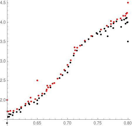
The application is that I have a costly function that tests whether $g(x,y)$ is true or false and it is known that if $g(x,y_1)$ is true so is $g(x,y_2)$ for all $y_2>y_1$. The goals is to find the (continuous) intersection $f(x)$.

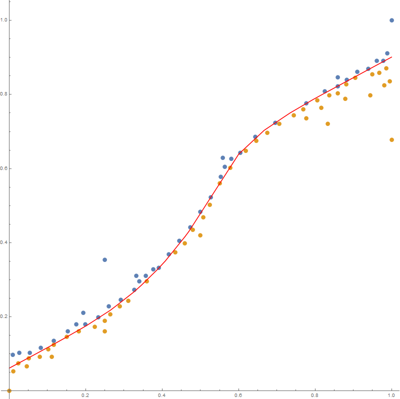
The following image should clarify the goal. The goal is to find the continuous curve between the black and the red dots.

Example


In general the shape of the interface will be to difficult to recognize as simple analytic function (or sum of analytic functions).

Monotonicity is not always guaranteed but I am already very interested in any solution assuming monotonicity of f(x).

$\endgroup$
6
  • 2
    $\begingroup$ Can you provide some additional context? What do the data points measure? What do the scales measure? Context may direct responders to solutions that have emerged in specific domains. Also, just curious ;-) $\endgroup$
    – Jagra
    Commented Nov 25, 2019 at 16:28
  • $\begingroup$ @Jagra, I don't think context would help a lot here. Except from the expectation that the intersection curve is continuous there is no expectation at all that it is a simple continuous function. I don't think there that it is useful to describe the origin. (If I give you the name of what is on the axes it won't mean anything to you unless you happen to be a physicist specialized in conformal field theory. But if your curiosity is really strong these results come from something called numerical conformal bootstrap. ) $\endgroup$
    – Kvothe
    Commented Nov 25, 2019 at 16:34
  • $\begingroup$ Is each point a "pair" of some kind? As in each black with each red point? Or are these simply two data sets of the same process $\endgroup$ Commented Nov 25, 2019 at 17:25
  • 3
    $\begingroup$ Despite what you say context is everything. A model just doesn't magically appear from looking at data. What can you say about the models that might generate such data? If you can't shed some light on the potential models, then it would seem that your criterion of success will be "I'll know it when I see it." $\endgroup$
    – JimB
    Commented Nov 25, 2019 at 17:55
  • 2
    $\begingroup$ If you knew the form of the lower curve and if the upper curve should be of the same form but just shifted upwards by a constant amount, then that would be the kind of "information" needed to help guide you. Otherwise, it's just a fishing expedition. Not that there's necessarily anything wrong with a fishing expedition when one is trying to figure out something at the beginning. But without some "context" it's just hard to know what to suggest. $\endgroup$
    – JimB
    Commented Nov 25, 2019 at 19:59

4 Answers 4

7
$\begingroup$

You can use FindMinimum to fit a smooth spline between these point sets.

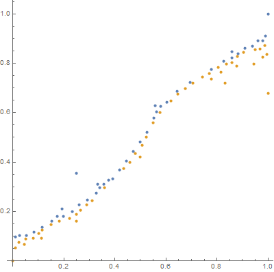
First of all, let's extract the red and black points in your image:

img = Import["https://i.sstatic.net/D0KpG.png"];
pts = ComponentMeasurements[
      Binarize[Erosion[ColorNegate[ColorDistance[img, #]], 1], .5], 
      "Centroid", #Circularity > .99 &][[All, 2]] & /@ {Red, Black};

I'm going to normalize all X/Y coordinates to 0..1 for clarity:

pts[[All, All, 1]] = Rescale[pts[[All, All, 1]]];
pts[[All, All, 2]] = Rescale[pts[[All, All, 2]]];    
{red, black} = pts;
ListPlot[pts, AspectRatio -> 1, ImageSize -> 400]

enter image description here

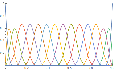
Next step: Let's define the spline that will fit between these two point sets. A spline is a sum of spline basis functions. I'll use 16 spline basis functions on the intervall [0..1]:

nVars = 16;
vars = c /@ Range[nVars];

degree = 3;
knots = Join[ConstantArray[0, degree], Subdivide[nVars - degree], 
   ConstantArray[1, degree]];

These basis functions look like this:

Plot[Evaluate[
  Table[BSplineBasis[{degree, knots}, i, x], {i, 0, nVars - 1}]], {x, 
  0, 1}, PlotRange -> All, ImageSize -> 400]

enter image description here

And the spline we're looking for is a weighted sum of these basis functions:

fn[x_] := 
 Table[BSplineBasis[{degree, knots}, i, x], {i, 0, nVars - 1}].vars

so e.g. fn[.3] evaluates to

0.000166667 c3 + 0.221167 c4 + 0.657167 c[6] + 0.1215 c[7]

The smoothness of the spline is simply:

smoothness = Total[Differences[vars, 2]^2];

(actually, I'm not sure this is 100% correct. I think the spacing of the knots should make a difference here. But since the knots are spaced equally between 0..1, it probably doesn't matter.)

And we have the constraint that the line should be above all black and below all red points:

constraints = 
 Flatten[{fn[#[[1]]] <= #[[2]] & /@ red, 
   fn[#[[1]]] >= #[[2]] & /@ black}];

Which leads to the simple optimization:

solution = FindMinimum[{smoothness, constraints}, vars]

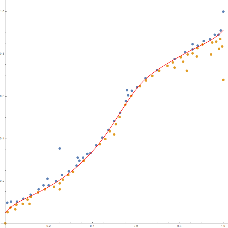
This takes a few seconds to evaluate, and if there is no spline with these knots that fits the constraints, FindMinimum will return an error. But for these points, and nVars=16, I get this nice looking solution:

Show[ListPlot[pts], 
 Plot[fn[x] /. solution[[2]], {x, 0, 1}, PlotStyle -> Red], 
 AspectRatio -> 1, ImageSize -> 400]

enter image description here

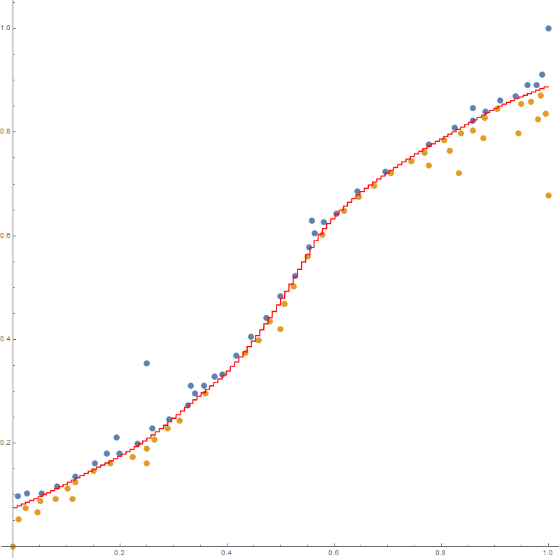
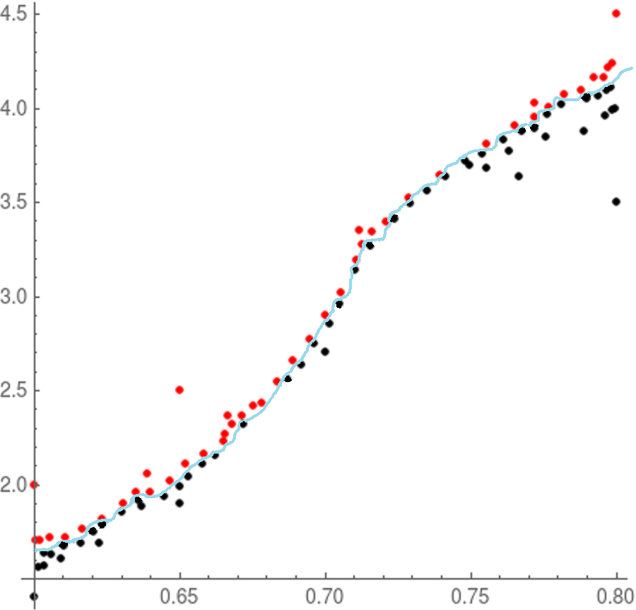
You can play with degree and nVars to get different curves. For example, for degree=0 and nVars=128, you get this piecewise-constant function:

enter image description here

and for degree=1, you get a piecewise linear function:

enter image description here

$\endgroup$
2
  • $\begingroup$ Thanks. This seems to work great for a small number of points. Unfortunately I am unable to make it work for a larger amount of points. I keep getting "There are no points that satisfy the constraints." I tried whether increasing nVars would help since the system is apparently over constraint but it did not. Any ideas how to make this solution scale well? $\endgroup$
    – Kvothe
    Commented Jan 14, 2020 at 11:04
  • $\begingroup$ @Kvothe: How many points are we talking about? You could use one control point for each constraint point, then there has to be solution. The optimization might be expensive, though. If you post a set of data points, I can play with it. $\endgroup$ Commented Jan 14, 2020 at 20:49
3
$\begingroup$

"I am already very interested in any solution assuming monotonicity of f(x)."

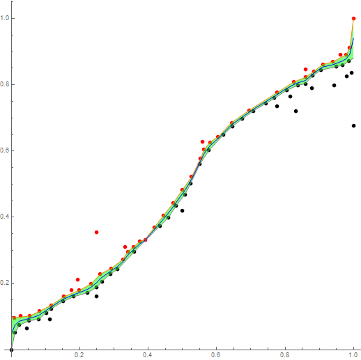
When the two lists are separable by a monotone curve (as is the case in OP) you can you can use Internal`List`Min twice to get the lower and upper envelopes, respectively, of the two lists.

Using the red and black from Niki's answer

{iFred, iFblack} = Interpolation[#, InterpolationOrder -> 1] & /@
     {{-1, 1} # & /@ SortBy[First][Internal`ListMin[{-1, 1} # & /@ red]],
      {1, -1} # & /@ SortBy[First][Internal`ListMin[{1, -1} # & /@ black]]}; 

Show[ListPlot[{red, black}, AspectRatio -> 1, 
    PlotStyle -> {Red, Black}, ImageSize -> Large], 
 Quiet @ Plot[{iFred[t], iFblack[t], (iFred[t] + iFblack[t])/2}, {t, 0, 1}, 
    AspectRatio -> 1, PlotStyle -> {Orange, Gray, Blue}, 
    Filling -> {1 -> {{2}, Opacity[.5, Green]}}]]

enter image description here

$\endgroup$
1
  • $\begingroup$ Thanks! This works great for a monotonic function. $\endgroup$
    – Kvothe
    Commented Jan 14, 2020 at 10:46
1
$\begingroup$

This is an extended comment rather than an answer.

Rather than performing two different regressions (one on the red dots and one on the black dots) and then determining what curve could fit between those curves, are you wanting to divide the area into "red" and "black" areas with the division being the curve you've labeled as $f(x)$? If so, that is more related to nonparametric discriminant analysis. (Although how the points are obtained is important which something you don't seem to want to describe.)

In short, are you looking for an automatic way to draw a curve between the red and black dots much as you would by eye? See below for such a curve.

Points with division line drawn by hand

$\endgroup$
0
$\begingroup$

(More of a comment in support of a previous answer.)

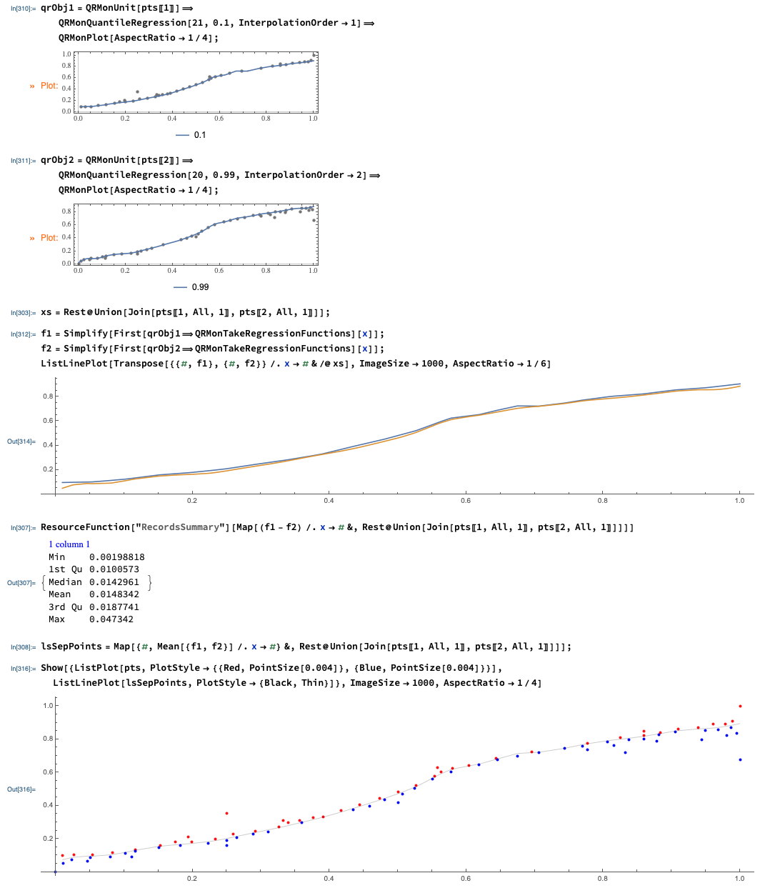
Using the plot data points obtained in Niki Estner answer and the software monad QRMon I was able to get the points of a curve that separates the plot data points.

enter image description here

Here are the points of the separation curve:

 lsSepPoints = {{0.00970874, 0.0734164}, {0.0107201, 0.074591}, {0.0230583,
   0.0862999}, {0.026699, 0.0888292}, {0.0461165, 
  0.0951937}, {0.0509709, 0.0949317}, {0.0533981, 
  0.0947557}, {0.0800971, 0.103061}, {0.0825243, 0.1044}, {0.101942, 
  0.118205}, {0.11165, 0.126589}, {0.116505, 0.130635}, {0.150485, 
  0.15415}, {0.152913, 0.15527}, {0.174757, 0.163744}, {0.182039, 
  0.166293}, {0.194175, 0.170232}, {0.199029, 0.171754}, {0.223301, 
  0.182906}, {0.23301, 0.188684}, {0.25, 0.201241}, {0.259709, 
  0.210016}, {0.264563, 0.214358}, {0.288835, 0.235617}, {0.291262, 
  0.237701}, {0.31068, 0.253775}, {0.326456, 0.267393}, {0.332524, 
  0.272801}, {0.339806, 0.279415}, {0.356796, 0.296439}, {0.359223, 
  0.298864}, {0.376214, 0.31558}, {0.390777, 0.330376}, {0.417476, 
  0.361744}, {0.434466, 0.382933}, {0.444175, 0.395235}, {0.458738, 
  0.41425}, {0.472896, 0.433024}, {0.480583, 0.443316}, {0.5, 
  0.471612}, {0.507282, 0.4826}, {0.524272, 0.510298}, {0.526699, 
  0.514491}, {0.550971, 0.566134}, {0.553398, 0.571524}, {0.558252, 
  0.581982}, {0.563107, 0.592012}, {0.57767, 0.618079}, {0.580097, 
  0.620602}, {0.604369, 0.640164}, {0.618932, 0.650728}, {0.643204, 
  0.678827}, {0.645631, 0.681975}, {0.674757, 0.714359}, {0.695388, 
  0.720076}, {0.706311, 0.721868}, {0.743932, 0.746009}, {0.769417, 
  0.767966}, {0.776699, 0.773092}, {0.805825, 0.791129}, {0.815534, 
  0.796254}, {0.825243, 0.800707}, {0.832524, 0.804183}, {0.837379, 
  0.806566}, {0.859223, 0.817977}, {0.878641, 0.831208}, {0.881068, 
  0.832888}, {0.883495, 0.834574}, {0.90534, 0.849879}, {0.910194, 
  0.852355}, {0.93932, 0.862786}, {0.944175, 0.863838}, {0.949029, 
  0.864693}, {0.961165, 0.86838}, {0.968447, 0.871859}, {0.978155, 
  0.877656}, {0.980583, 0.879313}, {0.98665, 0.883817}, {0.989078, 
  0.885763}, {0.995146, 0.890992}, {1., 0.895548}};
$\endgroup$

Your Answer

By clicking “Post Your Answer”, you agree to our terms of service and acknowledge you have read our privacy policy.

Not the answer you're looking for? Browse other questions tagged or ask your own question.