How to make a cow smaller (in BubbleChart3D plot)

Question

I've been using random walk Metropolis to sample from the (unnormalised distribution) which is defined as $p(r)\propto e^{-100 r}$, where $r$ is the perpendicular distance of a point in 3D space from the surface of the cow:

The code to do so is,

polygonCoords = Flatten[Cases[Normal[ExampleData[{"Geometry3D", "Cow"}]], 
Polygon[x_, ___] :> x, {0, Infinity}], 1];



fPDF[aPoint__, lPolygonCoords__] := Module[{aMin = 
                                    Min[EuclideanDistance[#, aPoint] & /@ lPolygonCoords]}, Exp[-100 aMin]]
fStep[aPoint__, aStepSize_] :=RandomVariate[MultinormalDistribution[aPoint, 
                                   aStepSize  IdentityMatrix[3]], {1}][[1]]
fAcceptStep[aPoint_, aStepSize_, lPolygonCoords__] :=  Module[{aProposed = fStep[aPoint, aStepSize], aRand = RandomReal[], r}, r = fPDF[aProposed, lPolygonCoords]/
fPDF[aPoint, lPolygonCoords]; If[r > aRand, aProposed, aPoint]]
fMetropolis[numSteps_Integer, aStart__, aStepSize_, lPolygonCoords__] := NestList[fAcceptStep[#, aStepSize, lPolygonCoords] &, aStart, numSteps]
data = Flatten[ParallelTable[
                           fMetropolis[1000, {0, 0, 0}, 0.001, polygonCoords], {i, 1, 4, 1}],1];

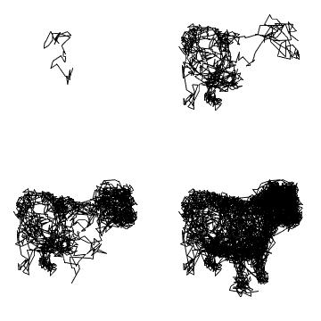
which generates sample paths over time that look like,

I want to draw a 3D point plot of all the sampled values where each of the points is a cow shape. I have tried doing this with,

n=10;
BubbleChart3D[
 Thread[{data[[1 ;; n, 1]], data[[1 ;; n, 2]], data[[1 ;; n, 3]], 
   ConstantArray[0.1, n]}], ChartElements -> aCow, 
 ChartStyle -> Black, BubbleSizes -> {0.02, 0.04}]

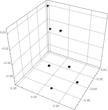
which does work for a small number of points (10 in the below case),

However, it does not scale well to 1000s of points, which is unsurprising given that each cow is a fairly complex 3D graphic. I have tried downsampling the cow's polygon coordinates and using these as markers instead by,

lRandomComponents = RandomInteger[{1, 5804}, 2000];

aLowResCow = 
 Graphics3D[{Opacity[1], EdgeForm[Opacity[1]], 
   Polygon[#, VertexColors -> Table[Hue[0, 0, 0], {Length[#]}]] & /@ 
    Cases[Normal[ExampleData[{"Geometry3D", "Cow"}]], 
      Polygon[x_, ___] :> x, {0, Infinity}][[lRandomComponents]]}]

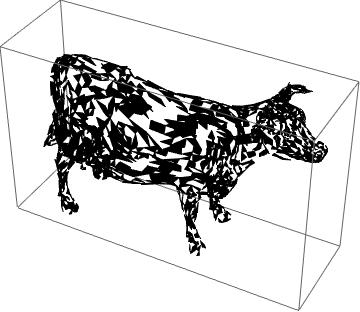
which generates a fragmented cow,

but using these doesn't really work on the BubbleChart3D plot (they are shaded grey -- I want them black -- and don't look much like cows).

Does anyone have any idea how I can generate a 3D point plot like what I want without having an enormous file size and taking my computer a day to produce? If it helps, I don't need to be able to rotate such a plot in 3D.

Answer 1

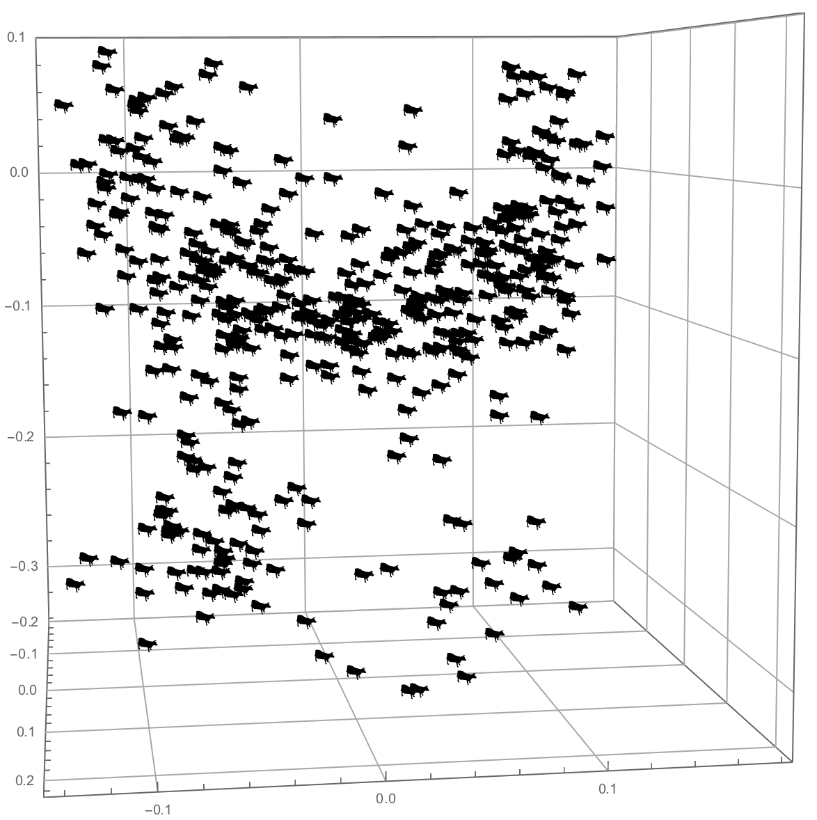
Here's a solution that can show 1000 cows using 1.45MB.

The idea is to project the 3D cow onto a 2D plane and then use this as the ChartElement with Inset. The advantage to using Inset is the face will not rotate when rotating the graphic.

To project into 2D, I approximate the shape for the sake of speed and size of the mesh.

Options[approximateProjectedMeshRegion] = {RasterSize -> Automatic, 
  "NumPoints" -> Automatic, Method -> Automatic};

approximateProjectedMeshRegion[mr_, vp_, OptionsPattern[]] :=
  Block[{n, num, rand, θ, bds, xd, yd, xmin, ymin, raw, im},
    n = Replace[OptionValue[RasterSize], Except[_Integer?Positive] -> 90, {0}];
    num = Replace[OptionValue["NumPoints"], Except[_Integer?Positive] -> 200000, {0}];

    rand = RandomPoint[mr, num];
    rand = RotationMatrix[{vp, {0, 0, 1}}].Transpose[rand];

    θ = VectorAngle[(RotationMatrix[{vp, {0,0,1}}].{0,0,1})[[1;;2]], {0, 1}];
    rand = Transpose[RotationMatrix[-θ].rand[[1;;2]]];

    bds = MinMax /@ Transpose[rand];
    {xd, yd} = Abs[Subtract @@@ bds]/n;
    {xmin, ymin} = bds[[All, 1]];

    raw = Transpose[{
        Clip[n+1 - Round[Divide[#2 - ymin, yd]], {1, n}],
        Clip[Round[Divide[#1 - xmin, xd]], {1, n}]
      }& @@ Transpose[rand]
    ];

    im = Image[SparseArray[Thread[Union[raw] -> 1]]];

    ImageMesh[im, Method -> OptionValue[Method], DataRange -> bds]
  ]

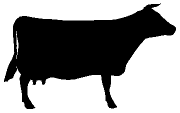
The approximated cow:

bmr2D = approximateProjectedMeshRegion[cow, {1.3, -2.4, 2.}]

This is a poor looking approximation, but that's ok. With 1000 cows, you won't notice the jagged corners. Moreover, it's small in size:

facepts = MeshPrimitives[bmr2D, 2][[1, 1]];
ByteCount[Graphics3D[Inset[Graphics[Polygon[facepts]]]]]

1328

Now unfortunately BubbleChart3D does not seem to accept Inset inside ChartElements, so we need to workaround. What we'll do is manually place the cows and use the options returned from BubbleChart3D.

n = 1000;
chartopts = Options[BubbleChart3D[Thread[{
  data[[1 ;; n, 1]], data[[1 ;; n, 2]], data[[1 ;; n, 3]], ConstantArray[0.1, n]}]
]];

scene = Graphics3D[
  Inset[Graphics[Polygon[facepts]], #, Center, 15] & /@ data[[1 ;; n]], 
  chartopts, 
  ImageSize -> Large
];

Here's its size:

ByteCount[scene]

1458864

Compare this to the size of 1000 cow's from ExampleData:

1000 ByteCount[ExampleData[{"Geometry3D", "Cow"}]]

1399072000

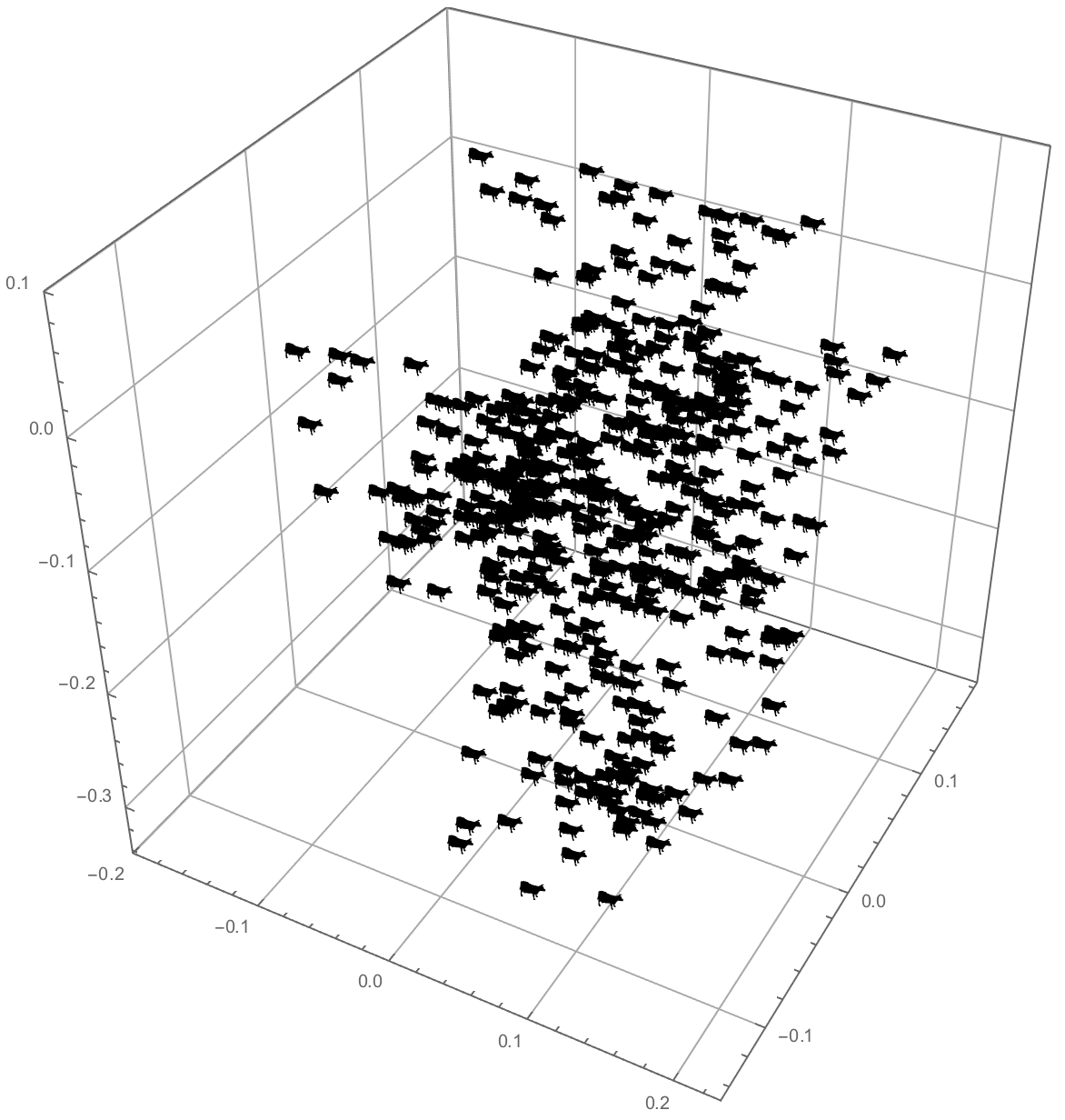
And here's the scene:

scene

And like I said earlier, if you rotate the graphic the cows will face the same direction:

Answer 2

I'm posting this just to demonstrate another method to get the cow's silhouette.

cow = ExampleData[{"Geometry3D", "Cow"}, "MeshRegion"];

Get the parameters for the projection plane:

cc = RegionCentroid[cow];
nrm = Flatten[Last[SingularValueDecomposition[
                   Standardize[MeshCoordinates[cow], Mean, 1 &], -1, Tolerance -> 0]]];

Now, pick out faces "above" the projection plane:

facs = Select[TranslationTransform[-cc] @@@ MeshPrimitives[cow, 2],
              VectorQ[#.nrm, Positive] &];

and transform those faces to the $x$-$y$ plane:

polys = Polygon[Composition[Drop[#, None, -1] &,
                            RotationTransform[{nrm, {0, 0, 1}}]] /@ facs];

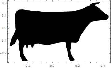
See the silhouette:

Graphics[polys]

To make an even simpler silhouette, we can cheat a little by rasterizing and then converting back to a polygon with ImageMesh[]:

cowPolygon = First[MeshPrimitives[ImageMesh[
   FillingTransform[ColorNegate[Binarize[Graphics[polys]]]],
   DataRange -> RegionBounds[polys]], 2]];

Graphics[cowPolygon, Frame -> True]

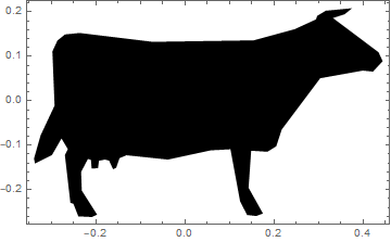
Even further simplification can be done by applying the Douglas-Peucker algorithm to this polygon. Using Szabolcs's SimplifyLine[]:

cowPolygon = Polygon[SimplifyLine[First[cowPolygon], 0.004]];

which yields

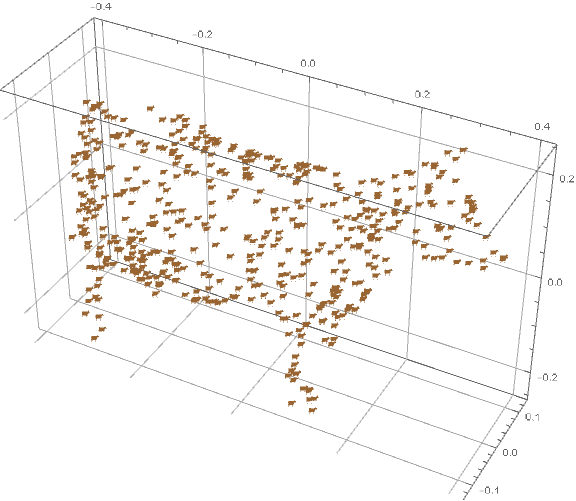
This can now be used in Inset[]. My computer is unable to evaluate the routines for generating the OP's points, so I'll use something different:

BlockRandom[SeedRandom[42]; pts = RandomPoint[cow, 500];]

Now, a scatter plot:

Graphics3D[Inset[Graphics[{Brown, cowPolygon}], #, Center, Scaled[0.015]] & /@ pts,
           Axes -> True, Boxed -> {Left, Bottom, Back}, 
           FaceGrids -> {{-1, 0, 0}, {0, 1, 0}, {0, 0, -1}}]