0
$\begingroup$

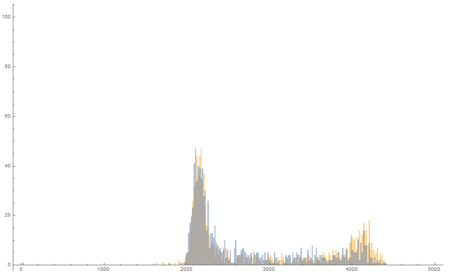
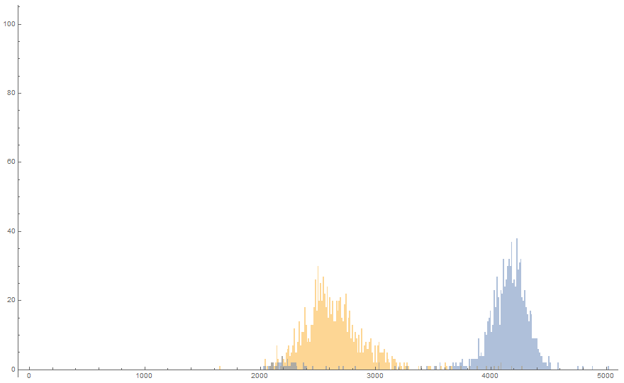
I have a series of data sets whose distributions I would like to quantitatively compare using Mathematica. For the purpose of this explanation, I will show two extreme comparisons (4 data sets total), where visually and experimentally the first comparison should show a greater dissimilarity than the second comparison.

Histogram[{t0sync[[1 ;; 1000]], 1.02 t8sync[[1 ;; 1000]]}, {"Raw", 500}, PlotRange -> {{0, 5000}, {0, 100}}]

Distribution Comparison 1

Histogram[{t0desync[[1 ;; 1000]], 1.02 t8desync[[1 ;; 1000]]}, {"Raw", 500}, PlotRange -> {{0, 5000}, {0, 100}}]

Distribution Comparison 2

DiscretePlot[{CDF[EmpiricalDistribution[t0sync[[1 ;; 1000]]], x], CDF[EmpiricalDistribution[1.02 t8sync[[1 ;; 1000]]], x]}, {x, 0, 5000}]

CDF Comparison 1

DiscretePlot[{CDF[EmpiricalDistribution[t0desync[[1 ;; 1000]]], x], CDF[EmpiricalDistribution[1.02 t8desync[[1 ;; 1000]]], x]}, {x, 0, 5000}]

CDF Comparison 2

Looking at the CDFs, I would expect the Kolmogorov-Smirnov Test of the first comparison should result in ~0.8 and the second comparison to result in ~0.1, but I am getting ~0 for both.

KolmogorovSmirnovTest[t0sync[[1 ;; 1000]], 1.02 t8sync[[1 ;; 1000]]]
3.069630061892*10^-375

KolmogorovSmirnovTest[t0desync[[1 ;; 1000]], 1.02 t8desync[[1 ;; 1000]]]
1.18559*10^-7

Does anyone have any insight as to why I'm getting these low of values when the CDFs indicate otherwise? Also, I'm not sure what is the easiest way to share the 4 datasets of 1000 points each for this example - please advise.

$\endgroup$
5
  • $\begingroup$ In the documentation for KolmogorovSmirnovTest, I don't see your usage: my understanding is that the second argument should be a distribution (e.g. LaplaceDistribution[1,2]). I don't see why you even get a result. $\endgroup$
    – anderstood
    Commented Mar 23, 2018 at 21:43
  • $\begingroup$ @anderstood The beginning/syntax part of the documentation doesn't list a KolmogorovSmirnovTest[data1, data2] option but that is given as one of the examples. Yes, that option should be made more explicit. $\endgroup$
    – JimB
    Commented Mar 23, 2018 at 22:06
  • 1
    $\begingroup$ The KolmogorovSmirnovTest returns a P-value which is close to zero for both. P-values are not of much use if you want to characterize the "size" of the difference between two distributions. A P-value just tells you the probability of seeing at least as extreme a sample difference in CDF's under the assumption that the samples are from the same distribution. That's usually not very interesting. You'd be better off to pick some summary statistics (mean, median, standard deviation, interquartile range, etc.) that have meaning to whatever subject matter you're dealing with and compare those. $\endgroup$
    – JimB
    Commented Mar 23, 2018 at 22:11
  • $\begingroup$ My intention is to generally characterize the differences more than just "size". If you look at the shape of the distributions, the typical statistical moments aren't telling as the distributions don't have statistically friendly shapes (at one point they are bi-modal and in another instance they have a single peak). I thought Kolmo-Smirnov would be the most appropriate for a general characterization, but maybe not. Thanks for taking the time to look at it. $\endgroup$
    – tquarton
    Commented Mar 24, 2018 at 0:30
  • 1
    $\begingroup$ By "size" I meant the value of any particular characterization of a difference (doesn't have to be a statistical moment). The Kolmogorov-Smirnov test statistic might not be a bad single-number summary statistic. Depends on what you need and the field of Statistics doesn't dictate your needs. That K-S statistic is estimating a quantity that doesn't change with sample size. But the P-value will tend to get smaller and smaller with increasing sample size. K-S statistic, fine. P-value, forget about it. But complex differences really need more than a single parameter for adequate description. $\endgroup$
    – JimB
    Commented Mar 24, 2018 at 1:50

1 Answer 1

4
$\begingroup$

If you have simple random samples from two distributions and want to characterize the difference in the underlying distributions with the Kolmogorov-Smirnov test statistic (the maximum difference in the cumulative distribution functions), then the following code will estimate that parameter and give approximate 95% confidence intervals for that parameter:

(* Generate samples from two distributions *)
nSamples1 = 400;
nSamples2 = 300;
data1 = RandomVariate[ChiSquareDistribution[10], nSamples1];
data2 = RandomVariate[ChiSquareDistribution[8], nSamples2];

(* Get K-S test statistic *)
ksObserved = KolmogorovSmirnovTest[data1, data2, "TestStatistic"]
(* 0.229167 *)

(* Perform a bootstrap that allows one to find approximate 95% confidence intervals *)
nboot = 1000;
ksBoot = ConstantArray[0, nboot];
Do[ksBoot[[i]] = KolmogorovSmirnovTest[RandomChoice[data1, nSamples1], 
   RandomChoice[data2, nSamples2], "TestStatistic"], {i, nboot}]
{lowerCL, upperCL} = {Quantile[ksBoot, 0.025], Quantile[ksBoot, 0.975]}
(* {0.165833, 0.308333} *)

You don't want to use the associated P-value for the K-S test as that quantity will tend to go to zero with large sample sizes if there is even any small difference between the two distributions.

$\endgroup$
1
  • $\begingroup$ Thanks JimB! I didn't realize the output was the P-value. I also appreciate the extra bootstrapping step. This was a very helpful answer. $\endgroup$
    – tquarton
    Commented Mar 27, 2018 at 16:19

Your Answer

By clicking “Post Your Answer”, you agree to our terms of service and acknowledge you have read our privacy policy.

Not the answer you're looking for? Browse other questions tagged or ask your own question.