Stochastic Lotka-Volterra Predator-Prey Model

Question

I am struggling with writing a stochastic version of Lotka-Volterra predator-prey model. This is as far as I have gotten:

a = 0.1;
b = 0.2;
c = 0.3;
d = 0.4;
proc = 
  RandomFunction[
    ItoProcess[
      {\[DifferentialD]X[t] == (a \[DifferentialD]t X[t] + \[DifferentialD]W[t]) - 
         b \[DifferentialD]t X[t] Y[t],
       \[DifferentialD]Y[t] == -c \[DifferentialD]t Y[t] + 
       d \[DifferentialD]t Y[t] X[t]}, 
      {X[t], Y[t]}, {{X, Y}, {0.2, 0.2}}, t, 
      W \[Distributed] WienerProcess[0, 0.1]], {0, 100, 0.01}, 
      Method -> "StochasticRungeKuttaScalarNoise"];
ListLinePlot[proc, PlotRange -> All]

For some reason, only one variable depends on the stochastic noise and it does not bear influence on the other part of the equation, I have tried to correct it, but no matter what I do, no luck.

First thing would be to get it working correctly, then I would worry about excluding "extinction Values > 0", since we are not interested in those.

Also, in regards to the graph, is there other way I would create a phase plot (X against Y)? My current way:

ListLinePlot[proc["Values"], PlotRange -> All]

plots X and Y, against time. How would I plot only X in time?

Answer 1

There are a few questions wrapped up here. Let me try to take them one-by-one.

only one variable depends on the stochastic noise and it does not bear influence on the other part of the equation

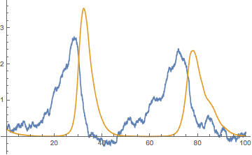
I don't think that's actually correct. After running your code,

ListLinePlot[proc, PlotRange -> All]

The predator (gold) seems to smooth over the variation in the prey (blue) but take a look around t=85: there is a random bump in prey which results in a little shoulder in the decline of the predators. So I think the simulation results are accurate for this model and parameter set.

then I would worry about excluding "extinction Values > 0", since we are not interested in those.

That prey can become negative is a problem with the model formulation. I don't think RandomFunction[ItoProcess has the equivalent of WhenEvent in NDSolve.

Two ideas: 1) replace your additive noise \[DifferentialD]W[t] with a multiplicative noise X[t] \[DifferentialD]W[t], which seems like it should prevent the prey population from becoming negative. 2) Instead of using a stochastic differential equation as your model, you could use a more basic continuous time stochastic process and simulate it with @IstvánZachar's GillespieSSA function from this answer (specifically, see his example 2).

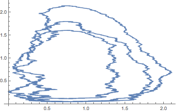
is there other way I would create a phase plot (X against Y)?

Funny, when I run your code, it works as desired (v11.2):

ListLinePlot[proc["Values"], PlotRange -> All]

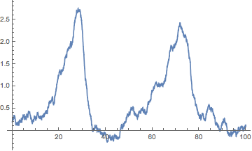
How would I plot only X in time?

This recent answer by @kglr addresses this point, using an undocumented property "PathComponent":

ListLinePlot[proc["PathComponent", 1]]

Anyone want to write a wrapper (call it SNDSolve) for RandomFunction[ItoProcess that mimics NDSolve in input and output? Seems like it'd be appreciated by many!

Answer 2

This solution will first define the ItoProcess and then simulate it; care is taken to initialize all the available parameters at their appropriate values (using With):

With[{a = 0.1, b = 0.2, c = 0.3, d = 0.4, Xo = 0.2, Yo = 0.2, wm = 0.,ws = 0.1},
 proc = ItoProcess[{
    \[DifferentialD]X[t] == (a - b Y[t]) X[t] \[DifferentialD]t + \[DifferentialD]W[t],
    \[DifferentialD]Y[t] == (-c + d X[t]) Y[t] \[DifferentialD]t
   }, {X[t], Y[t]}, {{X, Y}, {Xo, Yo}},
   t, W \[Distributed] WienerProcess[wm, ws]
  ]
 ];

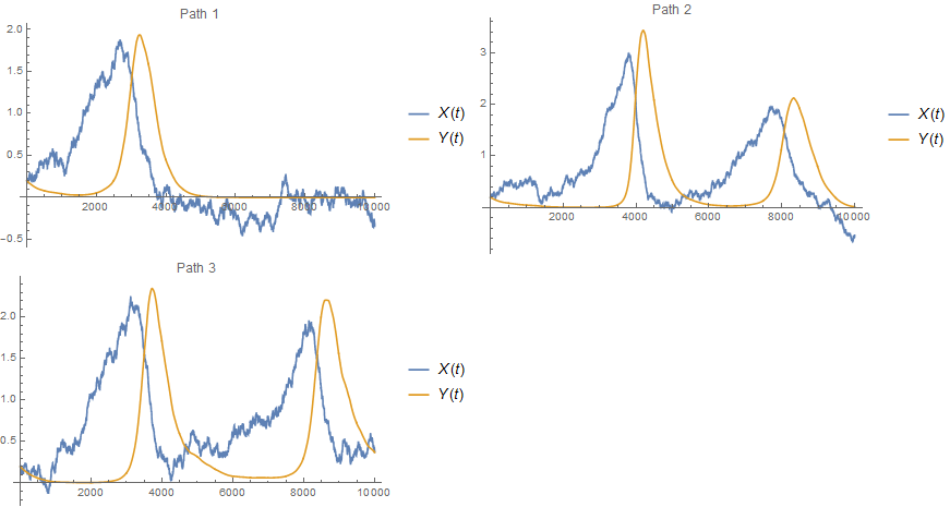
Next, we simulate 3 paths for the process (proc):

td = RandomFunction[proc, {0, 100, 0.01}, 3, Method -> "StochasticRungeKuttaScalarNoise"]

Finally we plot the derived paths:

Grid[
 Partition[
  MapIndexed[

   With[{val = Part[#1, All, -1]},
     ListLinePlot[
      Transpose[val],
      PlotRange -> All,
      PlotLegends -> {X[t], Y[t]},
      PlotLabel -> Row[{Path, Null, #2[[-1]]}]
    ]] &, td["Paths"]], 2, 2, {1, 1}, Null]]