How to calculate the first derivative from experimental data

Question

I have a set of experimental data and need to calculate the first derivative. What is the easiest way to do this? Many thanks in advance

Answer 1

You have a few options. If your data is not noisy at all it is much cleaner. When I say not noisy, you don't want a lot of random variation from $x_i$ to $x_{i+1}$. If you have that type of noise, you need to filter before you take the derivative.

clean data

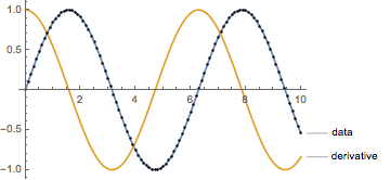
First up is simple interpolation and then take the derivative of the interpolating function.

SeedRandom[10];
x = Range[0, 10, .1];
y = Sin[x];
dat = Transpose[{x, y}];
int = Interpolation[dat];
p1 = ListPlot[dat, PlotStyle -> Black];
p2 = Plot[{int[x], int'[x]}, {x, 0, 10}, PlotLabels -> {"data", "derivative"}];
p3 = Show[{p2, p1}]

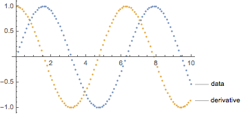
You can also do this numerically by taking the differences between each step. When you take the differences of the $y$ values, you'll want to divide through by $dx$. Also, your data is now one data point shorter, so you'll need to chop a value off of the $x$ values. You can be sloppy and just ignore the first or last point, or you can take the midpoint of each interval $(x_i + x_{i+1})/2$. The latter is more correct.

newx = Most[x] + Differences[x]/2;
newy = Differences[y]/Differences[x];
derivdat = Transpose[{newx, newy}];
p4 = ListPlot[{dat, derivdat}, Joined -> False, PlotLabels -> {"data", "derivative"}]

noisy data

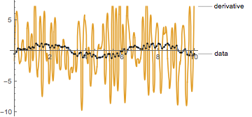
If you have noisy data, you have to work a little harder. The previous two methods still work, but you will need to filter the data before you take the derivative. For the interpolation method, you'll want to filter the data before you fit the interpolating curve. If you don't, you get something like the following mess.

ynoise = Sin[x] + RandomReal[{-.5, .5}, Length[x]];
datnoise = Transpose[{x, ynoise}];
int2 = Interpolation[datnoise];
p5 = ListPlot[datnoise, PlotStyle -> Black];
p6 = Plot[{int2[x], int2'[x]}, {x, 0, 10}, 
   PlotLabels -> {"data", "derivative"}];
p7 = Show[{p6, p5}]

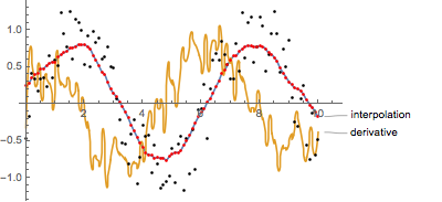
So smooth the data. MeanFilter and MedianFilter are good options. Pick a range that makes the curve smooth. 5-10 data points works for the toy data here. Also, note that if you put your data in a TimeSeries structure, it makes some of the manipulations a little more pleasant.

ysmoothed = MeanFilter[ynoise, 10];
datsmooth = Transpose[{x, ysmoothed}];
int3 = Interpolation[datsmooth];
p8 = ListPlot[{datnoise, datsmooth}, PlotStyle -> {Black, Red}];
p9 = Plot[{int3[x], int3'[x]}, {x, 0, 10}, 
   PlotLabels -> {"data", "derivative"}];
p10 = Show[{p9, p8}, PlotRange -> All, ImageSize -> 400]

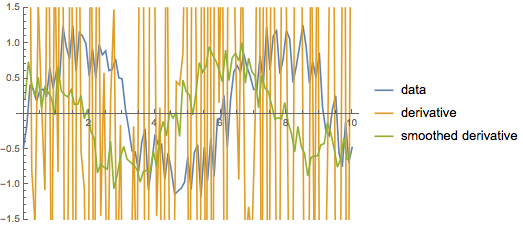
A similar thing occurs with the direct numerical derivative. Smooth it first.

newx2 = Most[x] + Differences[x]/2;
newy2 = Differences[ynoise]/Differences[x];
derivdat2 = Transpose[{newx2, newy2}];
newy3 = Differences[ysmoothed]/Differences[x];
derivdat3 = Transpose[{newx2, newy3}];
p11 = ListPlot[{datnoise, derivdat2, derivdat3}, 
  PlotLegends -> {"data", "derivative", "smoothed derivative"}, 
  Joined -> True, PlotRange -> {-1.5, 1.5}]

other filtering methods

If your data has data at repeated $x$ positions, you will need to treat it a bit differently, as Interpolation will choke and the simple numerical calculation will also have some issues. There are also implications if your data is unordered. One can construct various algorithms to these issues; I'll not address them here.

Two nice methods that address smoothing, multiple $x$ values, and unordered data are LOESS fitting and Savitzky-Golay filtering. I also won't go into a description of either of this here. LOESS fitting is not implemented in Mathematica, though is discussed here. Savitzky-Golay filtering is also not directly implemented, but can be roughed out very quickly using built in functions.

LOESS fitting

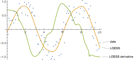
For the LOESS fitting, perform the fitting and then proceed with one of the two methods describe previously to get to the derivative. The interpolation method should work nicely. Note, I implemented a small LOESS package; it is not included in Mathematica. The package is here. All credit for the implementation goes to Rahul.

<< "Loess.wl"
fit = Loess[datnoise, 25, 1];
lfit = Transpose[{x, fit /@ x}];
int4 = Interpolation[lfit];
p12 = ListPlot[{datnoise, lfit}, Joined -> {False, True}, 
   PlotLabels -> {"data", "LOESS"}];
p13 = Plot[int4'[x], {x, 0, 10}, PlotStyle -> ColorData[97][3], 
   PlotLabels -> {"LOESS derivative"}];
p14 = Show[{p13, p12}, ImageSize -> 450]

Savitzky-Golay filtering

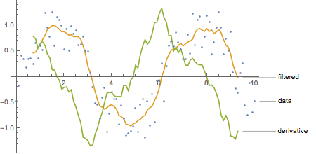
Savitzky-Golay filtering is implemented by convolving a kernel with the data. Specific kernels will give you a smoothed version of the convolved data or a derivative of the data. While the filtering technique is not implemented as a function, the kernels are accessible using SavitzkyGolayMatrix. I've not read too much into the theory of this filtering technique, but it probably requires regularly spaced data. Your filtered data will also be chopped short on either side based on your filter length. Longer filter lengths give you smoother data, but shorter results. You can also play with the degree of the polynomial in the filter (the 2nd argument to SavitzkyGolayMatrix); try and see what works best for your data.

Note, there is an amplitude change with filters that compute derivatives. Wikipedia says it is $n!/h^n$, where $n$ is the degree of the derivative and $h$ is interval between data points. I'm usually not concerned with this as I'm looking at the shape of the derivative and not the absolute scale.

derivscale = Factorial[1]/First[Differences[x]]^1;
filtlen = 7;
filt = SavitzkyGolayMatrix[{filtlen}, 2, 0];
filtderiv = SavitzkyGolayMatrix[{filtlen}, 2, 1];
sgx = x[[filtlen + 1 ;; -(filtlen + 1)]];
f1 = Transpose[{sgx, ListConvolve[filt, ynoise]}];
f2 = Transpose[{sgx, -derivscale*ListConvolve[filtderiv, ynoise]}];
p15 = ListPlot[{datnoise, f1, f2}, Joined -> {False, True, True}, 
  PlotLabels -> {"data", "filtered", "derivative"}, ImageSize -> 450]

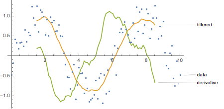
You can see changing the filter window and the degree of the filter can give you different results.

filtlen = 15;
filt = SavitzkyGolayMatrix[{filtlen}, 3, 0];
filtderiv = SavitzkyGolayMatrix[{filtlen}, 3, 1];
sgx = x[[filtlen + 1 ;; -(filtlen + 1)]];
f1 = Transpose[{sgx, ListConvolve[filt, ynoise]}];
f2 = Transpose[{sgx, -derivscale*ListConvolve[filtderiv, ynoise]}];
p16 = ListPlot[{datnoise, f1, f2}, Joined -> {False, True, True}, 
  PlotLabels -> {"data", "filtered", "derivative"}, ImageSize -> 450]