Dealing with derivative of noisy experimental data

Question

I have the following (time, position) dataset

  dataset = {{0, 0}, {0.0198413, 4.35004}, {0.0396825, 11.31}, {0.0595238, 
  17.4}, {0.0793651, 23.49}, {0.0992064, 26.97}, {0.238095, 
  66.99}, {0.257937, 73.08}, {0.277778, 78.3}, {0.297619, 
  84.39}, {0.31746, 91.35}, {0.337302, 95.7}, {0.357143, 
  102.66}, {0.376984, 106.14}, {0.396825, 112.23}, {0.416667, 
  118.32}, {0.436508, 124.41}, {0.456349, 131.37}, {0.47619, 
  138.33}, {0.496032, 145.29}, {0.515873, 150.51}, {0.535714, 
  156.6}, {0.555556, 162.69}, {0.575397, 168.78}, {0.595238, 
  175.74}, {0.615079, 180.09}, {0.634921, 187.05}, {0.654762, 
  192.27}, {0.674603, 198.36}, {0.694444, 203.58}, {0.714286, 
  210.54}, {0.734127, 214.02}, {0.753968, 220.98}, {0.77381, 
  227.07}, {0.793651, 233.16}, {0.813492, 239.25}, {0.833333, 
  243.6}, {0.853175, 248.82}, {0.873016, 254.91}, {0.892857, 
  260.13}, {0.912698, 264.48}, {0.93254, 272.31}, {0.952381, 
  275.79}, {0.972222, 281.01}, {0.992063, 286.23}, {1.0119, 
  294.06}, {1.03175, 298.41}, {1.05159, 303.63}, {1.07143, 
  308.85}, {1.09127, 314.94}, {1.11111, 319.29}, {1.13095, 
  324.51}, {1.15079, 329.73}, {1.42857, 388.02}, {1.44841, 
  393.24}, {1.46825, 396.72}, {1.50794, 410.64}, {1.52778, 
  411.51}, {1.5873, 421.95}, {1.60714, 425.43}, {1.62698, 
  428.91}, {1.64683, 429.78}, {1.66667, 432.39}, {1.68651, 
  435.87}, {1.70635, 439.35}, {1.72619, 442.83}, {1.74603, 
  448.05}, {1.76587, 452.4}, {1.78571, 456.75}, {1.80556, 
  460.23}, {1.8254, 464.58}, {1.84524, 467.19}, {1.86508, 
  469.8}, {1.88492, 471.54}, {1.90476, 474.15}, {1.9246, 
  475.89}, {1.94444, 479.37}, {1.96429, 481.98}, {1.98413, 
  486.33}, {2.00397, 488.94}, {2.02381, 492.42}, {2.04365, 
  495.03}, {2.06349, 498.51}, {2.08333, 501.12}, {2.10317, 
  504.6}, {2.12302, 507.21}, {2.14286, 508.95}, {2.1627, 
  512.43}, {2.18254, 515.91}, {2.20238, 518.52}, {2.22222, 
  522.}, {2.24206, 523.74}, {2.2619, 525.48}, {2.28175, 
  528.09}, {2.30159, 532.44}, {2.32143, 534.18}, {2.34127, 
  536.79}, {2.36111, 539.4}, {2.38095, 542.01}, {2.40079, 
  544.62}, {2.42063, 547.23}, {2.44048, 547.23}, {2.46032, 
  549.84}, {2.48016, 553.32}, {2.5, 555.93}, {2.51984, 
  558.54}, {2.53968, 559.41}, {2.55952, 562.02}, {2.57937, 
  563.76}, {2.59921, 566.37}, {2.61905, 568.11}, {2.63889, 
  571.59}, {2.65873, 573.33}, {2.67857, 577.68}, {2.69841, 
  577.68}, {2.87698, 595.08}, {2.89683, 596.82}, {2.91667, 
  598.56}, {2.93651, 601.17}, {2.95635, 603.78}, {2.97619, 
  606.39}, {2.99603, 607.26}}.

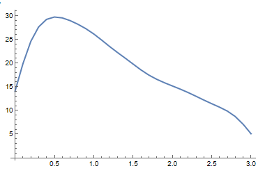
To my eyes they do not look very noisy. However, if I naively fit an interpolation curve and then differentiate

f = Interpolation[dataset, InterpolationOrder -> 3]
g = Interpolation[dataset, Method -> "Spline", InterpolationOrder -> 3]

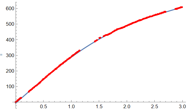
Show[ListPlot[dataset], Plot[f[t], {t, 0, 3}]]
Show[ListPlot[dataset], Plot[g[t], {t, 0, 3}]]

(*Derivative of interpolation function*)
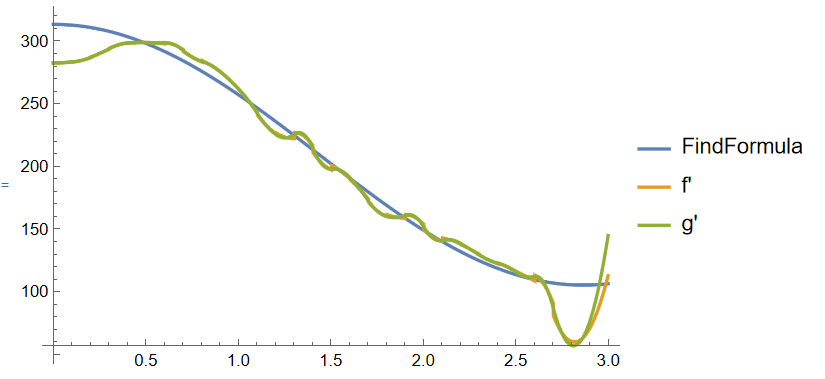
Plot[f'[t], {t, 0, 3}]
Plot[g'[t], {t, 0, 3}]

I produce a very noisy derivative.

I also tried a brute force numerical differentiation

(*Numerical derivative of data*)
newtime = Most[time] + Differences[time]/2;
newpos = Differences[pos]/Differences[time];
derivdat = Transpose[{newtime, newpos}];
p4 = ListPlot[{dataset, derivdat}, Joined -> False, 
  PlotLabels -> {"data", "derivative"}]

as well as smoothing the data first and then fitting an interpolation

(*Smooth data, then interpolation*)
possmoothed = MeanFilter[pos, 6]
datsmooth = Transpose[{time, possmoothed}];
int3 = Interpolation[datsmooth, Method -> "Spline", 
   InterpolationOrder -> 1];
p8 = ListPlot[{dataset, datsmooth}, PlotStyle -> {Black, Red}];
p9 = Plot[{int3[x], int3'[x]}, {x, 0, 3}, 
   PlotLabels -> {"data", "derivative"}];
p10 = Show[{p9, p8}, PlotRange -> All, ImageSize -> 400]

I am aware that I can obtain a good fit if I use a nonlinear model fit

nlm = NonlinearModelFit[dataset, a (1 - E^(-t/b)), {a, b}, t];

but I would like to have a method which works without assuming an underlying method (if possible). The reason being that in other datasets I expect the curve may have a point of inflection close to the center of the testing interval.

Answer 1

You don't describe the details of how the data was obtained. I suspect that any regression analysis should include accounting for serial correlation of observations over time.

But if that is not the case, you can use AIC (Akaike's Information Criterion) to select reasonable models. If you restrict yourself to polynomials (with no intercept as it appears from the first point being exactly (0,0)), then it appears that a 7-th degree polynomial is the best fit under that class of models as it has the lowest AICc value:

fit[p_] := LinearModelFit[dataset, Table[x^i, {i, p}], x, IncludeConstantBasis -> False]
TableForm[Table[{p, fit[p]["AICc"]}, {p, 1, 12}], 
 TableHeadings -> {None, {"Degree", "AICc"}}]

One of the advantages of a specific model (which ideally would come from theoretical reasons) is that you can obtain the derivative AND confidence bands for the derivative.

The estimated derivative and approximate lower and upper 95% confidence limits can be obtained in the following manner for a linear model:

dist = TransformedDistribution[Sum[a[i] x^(i - 1), {i, 1, 7}], 
  Table[a[i], {i, 1, 7}] \[Distributed] 
   MultinormalDistribution[fit[7]["BestFitParameters"], fit[7]["CovarianceMatrix"]]]
m = Mean[dist]
lower025 = Mean[dist] - 1.96*StandardDeviation[dist]
upper975 = Mean[dist] + 1.96*StandardDeviation[dist]
Plot[{lower025, upper975, m}, {x, 0, 3}, PlotStyle -> {LightGray, LightGray, Black}]

Answer 2

Differentiation amplifies noise, that's just the unfortunate reality. Unless you have a good "true model" of the data, all you can really do is smooth things out and hope for the best. In your case, it seems like it's best to treat the data like it's coming from an asymmetric function to reduce edge-effects around 0. TimeSeries is a good tool for this:

ts = TimeSeries[Join[-Rest[dataset], dataset]]
smoothedData = Normal@TimeSeriesResample[
    MeanFilter[ts, 0.25],
    0.1
 ];
f = Interpolation[smoothedData, InterpolationOrder -> 3]
g = Interpolation[smoothedData, Method -> "Spline", InterpolationOrder -> 3]

Plot[{f'[t], g'[t]} , {t, 0, 3}]

Answer 3

There are no universal method for any data set. But in this case we can get a good fit with

FindFormula[dataset, t]
-6.11193 + 211.614 t + 11.0887 t Cos[t] + 90.5696 Sin[t]

Visualization

Show[Plot[%, {t, 0, 3}], ListPlot[dataset, PlotStyle -> Red]]

Therefore first derivative is

d1=211.614 + 101.658 Cos[t] - 11.0887 t Sin[t]

Now we can use smoothing data from the code proposed by Sjoerd Smit

Plot[{d1, f'[t], g'[t]}, {t, 0, 3}, 
 PlotLegends -> {"FindFormula", "f'", "g'"}]

Answer 4

Here is a strategy to achieve your aim using digital filters.

First we need to create a new dataset with equidistant points. This can be achieved by fitting some curve to the data, here I am using "Interpolation". With the help of this, we create equidistant data points:

fun = Interpolation[dataset];
dat = Table[{x,fun[x]}, {x, 0, 3, 0.1}];

Now we can use a digital filter that calculates the derivatives and at the same time smoothes the data and acts on the y values. Here I am using "DerivativeFilter". The smoothing strength can be adjusted by the last argument:

datd = DerivativeFilter[dat[[All, 2]], {1}, 2];

To get the correct x scale, we must add the x coordinates
again:

datd = Transpose[{dat[[All, 1]], datd}];
ListLinePlot[datd]