5
$\begingroup$
F = Sqrt[x^2+(y + I/2)^2];

Plot3D[Im[F], {x, 0, 1}, {y, -1, 1}, 
AxesLabel -> Automatic, 
Mesh -> None, 
ColorFunction -> Function[{x, y, z}, ColorData["TemperatureMap"][z + 0.5]],  
ColorFunctionScaling -> False, 
ViewPoint -> {2, -2, 1.5}]

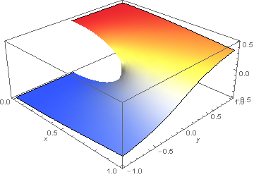
enter image description here

This plot is fine. However, when I want to plot the figure below:

Plot3D[{Im[F],-Im[F]}, {x, 0, 1}, {y, -1, 1}, 
AxesLabel -> Automatic, 
Mesh -> None, 
ColorFunction -> Function[{x, y, z}, ColorData["TemperatureMap"][z + 0.5]],  
ColorFunctionScaling -> False, 
ViewPoint -> {2, -2, 1.5}]

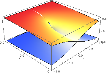
enter image description here

There is a gap in the upper surface (the white line). Is there any way to remove the gap to make the upper surface smooth?

Maybe one solution is to use Piecewise to rewrite the function for the upper surface. However, I don't want yo use this method, because my further project needs to plot 4 such surfaces, which is difficult to use Piecewise.

Another solution is using "Exclusions -> None". However, when the figure is rotated, the figure is bad.

Any good solutions?

$\endgroup$

3 Answers 3

7
$\begingroup$

Warning: dirty hacky solution ahead

Just take the y values that are close to zero and make them equal to zero. If plot is defined as in the OP, then

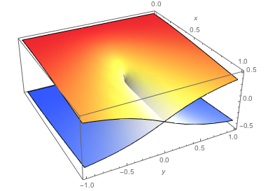
plot /. {x_Real, y_Real, z_Real} :> {x, Chop[y, .01], z}

Mathematica graphics

$\endgroup$
2
  • 1
    $\begingroup$ What is the definition of plot and what is OP? $\endgroup$
    – Qi Zhong
    Commented May 9, 2017 at 19:52
  • 1
    $\begingroup$ @QiZhong OP = "original post", i.e. plot refers to the Plot3D code you used. $\endgroup$
    – user170231
    Commented May 9, 2017 at 20:31
6
$\begingroup$

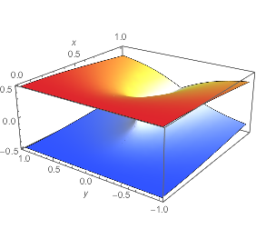
You could use ContourPlot3D:

ContourPlot3D[z^2 == Im[F]^2, {x, 0, 1}, {y, -1, 1}, {z, -0.5, 0.5}, 
  AxesLabel -> Automatic, Mesh -> None, 
  ColorFunction -> Function[{x, y, z}, ColorData["TemperatureMap"][z + 0.5]], 
  ColorFunctionScaling -> False, ViewPoint -> {2, -2, 1.5}, 
  BoxRatios -> {1, 1, 0.4}]

enter image description here

$\endgroup$
1
  • $\begingroup$ This can work. But one disadvantage: it seems this method will use longer CPU time. And I can feel the display is not smooth(it needs time to run the code) when I rotate the figure, compared with using Plot3D. $\endgroup$
    – Qi Zhong
    Commented May 9, 2017 at 19:56
2
$\begingroup$

A dirty hack would be to draw two parametric stripes along the exclusions with the same coloring:

F[x_?NumericQ, y_?NumericQ] := Im@Sqrt[x^2 + (y + I/2)^2]

Show[
 Plot3D[{F[x, y], -F[x, y]}, {x, 0, 1}, {y, -1, 1}, 
  AxesLabel -> Automatic, Mesh -> None, 
  ColorFunction -> 
   Function[{x, y, z}, ColorData["TemperatureMap"][z + 0.5]], 
  ColorFunctionScaling -> False, ViewPoint -> {2, -2, 1.5}, 
  Exclusions -> y == 0],
 ParametricPlot3D[{x, y, F[x, 0]}, {x, 0, 1}, {y, -0.01, 0.01}, 
  Mesh -> None, 
  ColorFunction -> 
   Function[{x}, ColorData["TemperatureMap"][F[x, 0] + 0.5]], 
  ColorFunctionScaling -> False, Exclusions -> None],
 ParametricPlot3D[{x, y, -F[x, 0]}, {x, 0, 1}, {y, -0.01, 0.01}, 
  Mesh -> None, 
  ColorFunction -> 
   Function[{x}, ColorData["TemperatureMap"][-F[x, 0] + 0.5]], 
  ColorFunctionScaling -> False, Exclusions -> None]
 ]

enter image description here

$\endgroup$

Your Answer

By clicking “Post Your Answer”, you agree to our terms of service and acknowledge you have read our privacy policy.

Not the answer you're looking for? Browse other questions tagged or ask your own question.