Fitting Asymptotic Ansatz to Numerical solution of Differential equation

Question

Consider the following differential equation: $$ \frac{1}{a} \frac{dy}{dx} = -\frac{1}{y} e^{-\frac{1}{y}} $$ with initial condition $y(0) = 1$ and $a = 10$. This is easily solved numerically with $Mathematica$ and I can also solve this analytically in the limit $x\to \infty$ to get the asymptotic behavior $$ y(x) \sim \frac{1}{\log(a x)} $$ Is there a way I can use fit this asymptotic tail to the numerical solution? I tried this ansatz but I couldn't figure out the best way to show that indeed the numerical solution has this logarithmic tail.

Edit: I realize now the question was misleading. What I meant was, I know there is a logarithmic tail but I'm not certain what it's exact form is i.e., I want to fit the tail with the ansatz $$\frac{c}{\log(k\,a\,x)}$$ where $c,k$ are unknown.

Answer 1

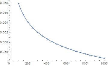
The updated equation for the form of the tail does seem to fit the differential equation quite well. First solving the differential equation yields:

sol=With[{a=10},NDSolve[{1/a*y'[x]==-1/y[x]*Exp[-1/y[x]],y[0]==1},y[x],{x,0,1000}]]

Next, evaluate the solution found by NDSolve for some time points in the tail.

data=Table[{i,Evaluate[y[x]/.sol[[1]]]/.x->i},{i,100,1000}];

Now solve for the form of the tail behavior

nlm = With[{a=10} , NonlinearModelFit[data, c/Log[k*a*x], {c, k}, x]
(*FittedModel[0.797369/Log[1263.96 x]]*)

Now check the goodness of our fitting

nlm["RSquared"]
(*1.*)

Visually checking our fitted model

Show[ListPlot[data2], Plot[nlm[x], {x, 100, 1000}]]

Answer 2

What you can do is , separate your differential equation in one part only dependent of y and the other part (side) only dependent of x and than integrate both sides. You then get a function for x here called xs dependent of y. This can not be solved with Solve to y[x], but you can Plot it with ParametricPlot or with FindRoot find the y for a given x. By the way, the aproximation 1/Log[a x] is not very good.

    In[14]:= xs[y_] = 
Integrate[(-1/10) ys Exp[1/ys], {ys, 1, y}, Assumptions -> y > 0]

Out[14]= 1/20 (2 E - E^(1/y) y (1 + y) - ExpIntegralEi[1] + 
ExpIntegralEi[1/y])

In[15]:= Solve[xs[y] == x, y]

During evaluation of In[15]:= Solve::nsmet: This system cannot be    solved with the methods available to Solve. >>

 In[77]:= Solve[y == 1/Log[10 x], x]

 Out[77]= {{x -> E^(1/y)/10}}

  In[86]:= ParametricPlot[{{xs[y], y}, {E^(1/y)/10, y}}, {y, 0.001,   1}, 
   PlotRange -> {{0, 100}, {0, 1}}, AspectRatio -> 1, 
   MaxRecursion -> 10, PlotStyle -> {Blue, Red}]

 In[25]:= yf[x_] := y /. First@FindRoot[xs[y] == x, {y, .1}]

   In[89]:= Plot[yf[x], {x, 0, 10}, PlotRange -> {0, 1}]

Continuing my answer:

Your Ansatz c/Log[a kx] for the tail of your solution is quite bad. For very large x it yields errors up to 15 percent and higher. See:

    In[1]:= dgl = 1/10 D[y[x], x] == - 1/y[x] Exp[-1/y[x]]

    In[75]:= ynd[x_] = 
     y[x] /. First@NDSolve[dgl && y[0] == 1, y, {x, 0, 10000000000}]



      In[77]:= {cf, 
     kf} = ({c, k} /. 
    FindRoot[
      ynd[1000] == 
          c/Log[10 k 1000] && (D[c/Log[10 k x], x] /. 
          x -> 1000) == -10 E^(-(1/ynd[1000]))/ynd[1000], {{c, 1}, {k, 
        1}}])

   Out[77]= {0.814938, 171.023}

   In[79]:= ypw[x_] = 
   Piecewise[{{ynd[x], 0 <= x <= 1000}, {cf/Log[10 kf x], x > 1000}}]

    In[80]:= Plot[(ypw[x]/ynd[x] - 1) 100, {x, 0, 10000000000}, 
     PlotRange -> All]

     In[81]:= xs[y_] = 
     Integrate[(-1/10) ys Exp[1/ys], {ys, 1, y}, Assumptions -> y > 0]          // 
      Expand

       Out[81]= E/10 - 1/20 E^(1/y) y - 1/20 E^(1/y) y^2 - 
   ExpIntegralEi[1]/20 + 1/20 ExpIntegralEi[1/y]

    In[96]:= yf[x_?NumericQ] := 
    y /. First@FindRoot[xs[y] == x, {y, 10^-6, 1}, WorkingPrecision ->   50]

     In[131]:= Plot[(ypw[x]/yf[Rationalize[x, 0]] - 1) 100, {x, 0, 
    10000000000}, PlotRange -> All]

    In[129]:= LogLinearPlot[(ypw[x]/yf[Rationalize[x, 0]] - 1) 100,   {x,   1,
    10^400}, PlotRange -> All]