Numerical bounce solution

Question

I want to solve numerically the following differential equation

$$ y''(x) + \frac{3}{x}y'(x) = \frac{d U(y)}{y}\,,\qquad U(y) = \frac{1}{4}y(x)^2(y(x)-1)^2 -\frac{1}{400}y(x)^3 $$

in the region $x\in[0,+\infty]$ with the bounce boundary conditions

$$ y'(0) = 0\,,\qquad y(+\infty) = 0. $$

This problem is taken from Coleman's paper (click here) where he claims that such solution always exists, see page 4, right-column independently of the expression of the potential $U(y)$.

I want to find such solution for the potential that I have chosen.

This is a boundary-values problem and it is better to turn it into a initial-values problem. Let us then estimate the size of $y(0)$. It will become clear that I expect a flat direction around $x=0$, so substituting $y'(0)=0$ and $y''(0) = 0$ in the differential equation, I get an estimate for the initial condition $y(0) \sim 1$. This is just an estimate. I don't want the exact solution to satisfy $y''(0)=0$ identically, but I expect the second derivative to be small.

We can try to guess the form of the solution by making some approximations. Indeed, I can solve analytically the differential equation for big values of $x\geq R \gg 1$, by neglecting the $1/400y(x)^3$ term in the expression of $U(y)$, as $y(0) \sim 1$ and $y(+\infty) = 0$; then, by defining $U_0(y) = \frac{1}{4}y(x)^2(y(x)-1)^2$ we can solve

$$ y''(x)= \frac{d U_0(y)}{y}\, $$

from which we get

$$ y_R(x) = \frac{1}{2}\left(1-\text{tanh}\left[\frac{x-R}{2\sqrt{2}}\right]\right). $$

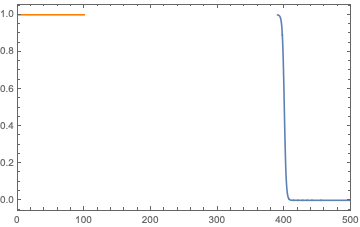
So, roughly the approximated solution is

$$ y(x) = \left\{\begin{array}{c c} 1 & x \ll R\\ y_R(x) & x \geq R \end{array}\right. $$ and it is shown in the following picture for $R=400$

So, I have tried to solve numerically this Cauchy problem without any approximation by setting a cut-off $R$ on the $x$ coordinates and using the following code

V[y_[x_]] = 1/4 (-1 + y[x])^2 y[x]^2 - 0.0025 y[x]^3

Psol = ParametricNDSolveValue[{D[y[x], {x, 2}] + 3/x D[y[x], x] == D[V[y[x]], y[x]], y'[10^-5] == 0, y[10^-5] == tp, WhenEvent[y[x] < 0 || y[x] > tp, "StopIntegration"]}, y, {x, 10^-5, R}, {tp, R}]

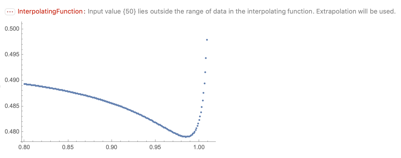
ListPlot[Table[{tp, Abs[Psol[tp, 50][50]]}, {tp, 0.8, 1.015, 0.001}]]

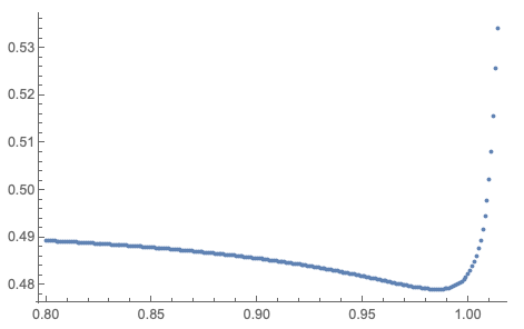
where the last line may be useful to determine the magnitude of tp such that I recover a vanishing asymptotic value. However, I get the following plot

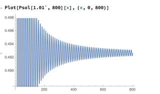
So, I guess the method is not suitable for this problem. In particular, the solution Mathematica finds does not respect the asymptotic boundary condition $y(+\infty) = 0$ at $x=50$, and moreover it starts oscillating after some time like in the following picture and does not go to zero at infinity

How can I get the numerical solution?

Answer 1

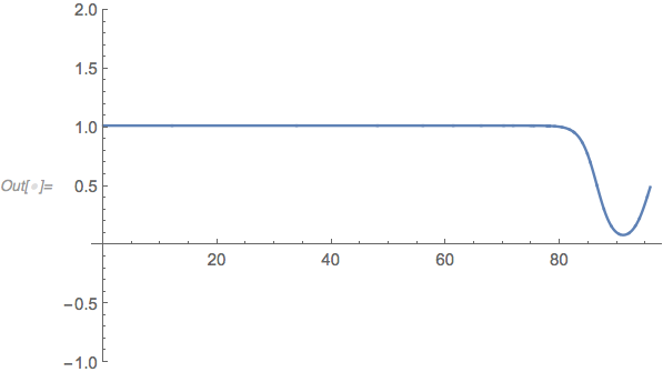
The argument in the paper linked in the comments suggests that if one starts close enough to the one equilbrium at $y \approx c_1 = 1.04$, then the asymptotically vanishing solution may be found. Below is a solution that is not quite there. It starts at $x = 10^{-8}$ at $y = c_1 - 10^{-25}$ and uses WorkingPrecision -> 50; it certainly needs more than machine precision to ensure that $y$ does not round to $c_1$. It's not close enough. Getting close enough seems to require a very small difference and consequently a very high working precisions. But NDSolve fails when I push it, indicating an error test failure (NDSolveValue::nderr). It may be that for such an example to be computationally feasible, you need a greater difference in the value of V[x] at the minima.

ClearAll[V];
V[y_] = 1/4 (-1 + y)^2 y^2 - 25/10000 y^3;
ode = y''[x] + (3 y'[x])/x == V'[y[x]];

wp = 50;
cps = NSolve[V'[y] == 0, WorkingPrecision -> wp];

ndsol[x0_?NumericQ, x1_?NumericQ, y0_?NumericQ, yp_?NumericQ] := 
  NDSolveValue[{ode, y'[x1] == yp, y[x1] == y0, 
    WhenEvent[y[x] < 0, "StopIntegration"],
    WhenEvent[y[x] > 49/100 && x > x1, "StopIntegration"]}, 
   y, {x, x0, 10000}, 
   WorkingPrecision -> Precision@{x0, x1, y0, yp}];
ListLinePlot[
 ndsol[2^-50, 1/10^8, y - 10^-25 /. Last@cps, 0],
 PlotRange -> {All, {-1, 2}}]

---

Update

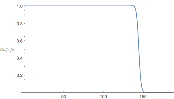
Here is a better result, FWIW. The method "Extrapolation" is more robust on this problem.

wp = 150;  (* working precision *)
cps = NSolve[V'[y] == 0, WorkingPrecision -> wp]; 
iObj[x0_?NumericQ, x1_?NumericQ, y0_?NumericQ, yp_?NumericQ] := 
 Catch@NDSolveValue[{ode, y'[x1] == yp, y[x1] == y0, 
    WhenEvent[y[x] < 0, Throw[x]],
    WhenEvent[y[x] > 49/100 && x > x1, Throw[$Failed]],
    WhenEvent[y[x] > 2 && x > x1, Throw[$Failed]]}, y, {x, x0, 1000}, 
   WorkingPrecision -> Precision@{x0, x1, y0, yp}, 
   Method -> "Extrapolation"];
obj[dy_?NumericQ] := iObj[2^-50, 1/10^8, y - 10^dy /. Last@cps, 0];

foo = Nest[  (* bisection method for finding optimal IC *)
  With[{mid = obj[Mean@#]},
    Switch[mid,
     $Failed, {First@#, Mean@#},
     _?NumericQ, {Mean@#, Last@#},
     _, {First@#, Mean@#}
     ]
    ] &,
  {-42 - 54/100, -42 - 53/100},
  60
  ]
(*
  {-(2452178951689226635963/57646075230342348800), 
   -(196174316135138130877/4611686018427387904)}
 *)
ndsol[x0_?NumericQ, x1_?NumericQ, y0_?NumericQ, yp_?NumericQ] := 
  NDSolveValue[{ode, y'[x1] == yp, y[x1] == y0, 
    WhenEvent[y[x] < 0, "StopIntegration"],
    WhenEvent[y[x] > 49/100 && x > x1, "StopIntegration"],
    WhenEvent[y[x] > 2 && x > x1, "StopIntegration"]}, 
   y, {x, x0, 10000}, WorkingPrecision -> Precision@{x0, x1, y0, yp}, 
   Method -> "Extrapolation"];
ListLinePlot[
 ndsol[2^-50, 1/10^8, y - 10^dy /. Last@cps, 0] /. dy -> First@foo,
 PlotRange -> All]

Answer 2

(Not an answer, an extended comment.)

So, I guess the method is not suitable for this problem. How can I get the numerical solution??"

Those statement and question do not make much sense to me. You already have the numerical solution. Why do you think the method is not suitable? The message InterpolationFunction::dmval is avoided if you decrease the range of tp a little (with 0.001). Study this result plot:

ListPlot[Table[{tp, Abs[Psol[tp, 50][50]]}, {tp, 0.8, 1.014, 0.001}], PlotRange -> All]

Also, maybe you should study the solution behavior for different values of the independent variable x not just 50.

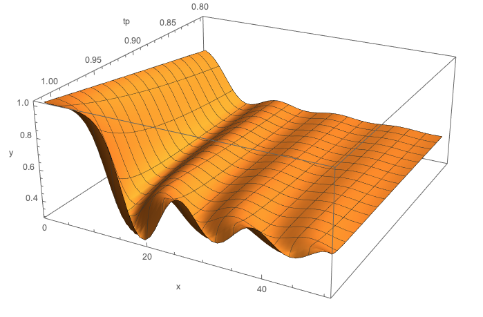
For example, the following 3D plot gives an idea of the found solution behavior with respect to both tp and x. (We can see the "bouncing" along the x-axis.)

points = Flatten[Table[{tp, x, Abs[Psol[tp, 50][x]]}, {tp, 0.8, 1.014, 0.001}, {x, 1, 50, 1}], 1];
ListPlot3D[points, AxesLabel -> {"tp", "x", "y"}, PlotRange -> All]

Answer 3

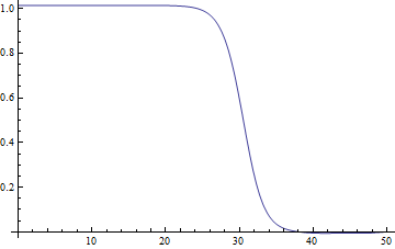
OK, Michael E2's answer gives me the courage to post the following as an answer. It seems that finite difference method (FDM) can be used to find the solutions for this problem in a relatively easy way. I'll use pdetoae for the generation of finite difference equations:

Clear[V];
V[y_] = 1/4 (-1 + y)^2 y^2 - 25/10000 y^3;
ode = y''[x] + (3 y'[x])/x == V'[y[x]];    
newode = # x & /@ ode // Simplify
inf = 50;
domain = {0, inf};
bc = {y'[0] == 0, y[inf] == 0};
points = 500;
difforder = 2;
grid = Array[# &, points, domain];
(* Definition of pdetoae isn't included in this post,
   please find it in the link above. *)
ptoafunc = pdetoae[y[x], grid, difforder];
ae = ptoafunc[newode][[2 ;; -2]];
aebc = ptoafunc@bc;

initial[x_] := 2;
sollst = FindRoot[{ae, aebc}, Table[{y@x, initial@x}, {x, grid}]][[All, -1]];
ListLinePlot[sollst, DataRange -> domain]
sol = ListInterpolation[sollst, grid];
(* Error check: *)
Plot[Subtract @@ ode /. y -> sol // Evaluate, {x, 0, inf}, PlotRange -> All]

I hesitated to post this because:

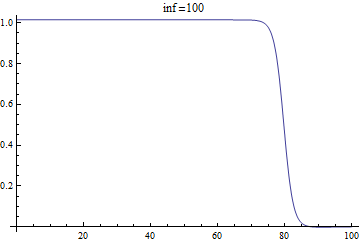
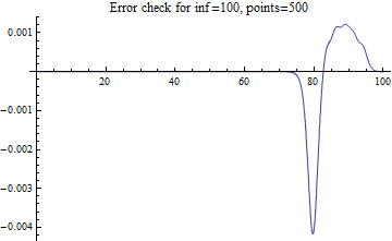
1. Using different inf, I can find different solutions, e.g. inf = 100:

2. The error of the solution isn't that small, and even if I increase points, I cannot observe obvious error reduction:

   

But now, reading all the analysis above, I believe there just exist multiple solutions for the problem, and the code above is worth sharing.