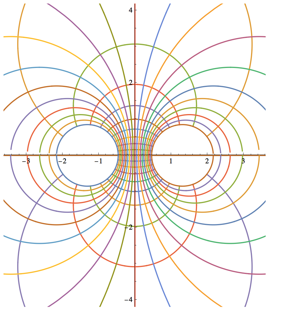
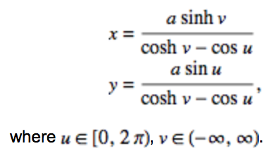
What you tried is the syntax for a parametric surface. However, you want to plot the coordinate lines. This can be done by stepping through one of the coordinate ranges in discrete steps and plotting a continuous parametric line by varying the other coordinate:
Show[ParametricPlot[
  Evaluate[Table[
    Tooltip[{Sinh[v]/(Cosh[v] - Cos[u]), Sin[u]/(Cosh[v] - Cos[u])},
     Row[{"u \[LongEqual] ", u}]], {u, 0, 2 Pi, Pi/10}]], {v, -1, 1}],
  ParametricPlot[
  Evaluate[Table[
    Tooltip[{Sinh[v]/(Cosh[v] - Cos[u]), Sin[u]/(Cosh[v] - Cos[u])},
     Row[{"v \[LongEqual] ", v}]], {v, -1, 1, 1/10}]], {u, Pi/100,
   2 Pi}]]

Here I did one ParametricPlot for each family of coordinate lines. In each ParametricPlot, the family of lines is generated by specifying the argument as a Table. One of the variables is the index of the table, so it's discrete, and the other variable is being used as the plot parameter.
I add Evaluate in front of the Table so that the list entries with different discrete indices are generated before being passed to ParametricPlot. This is something you have to do whenever using a Plot related command that has attribute HoldAll. If you omit the Evaluate, all lines generated in the Table will be plotted with the same color.
You may also be interested in the built-in functionality that can be accessed through things like this:
CoordinateTransformData[
 "BipolarCylindrical" -> "Cartesian", "Mapping", {u, v, z}]
Edit
To help explain the coordinate system, it's useful to label each colored line by the fixed parameter it corresponds to. I did this using Tooltip. So if you now hover over any of the lines, the tooltip will appear and tell you which coordinate was held constant to make that curve, and what value it was held at.


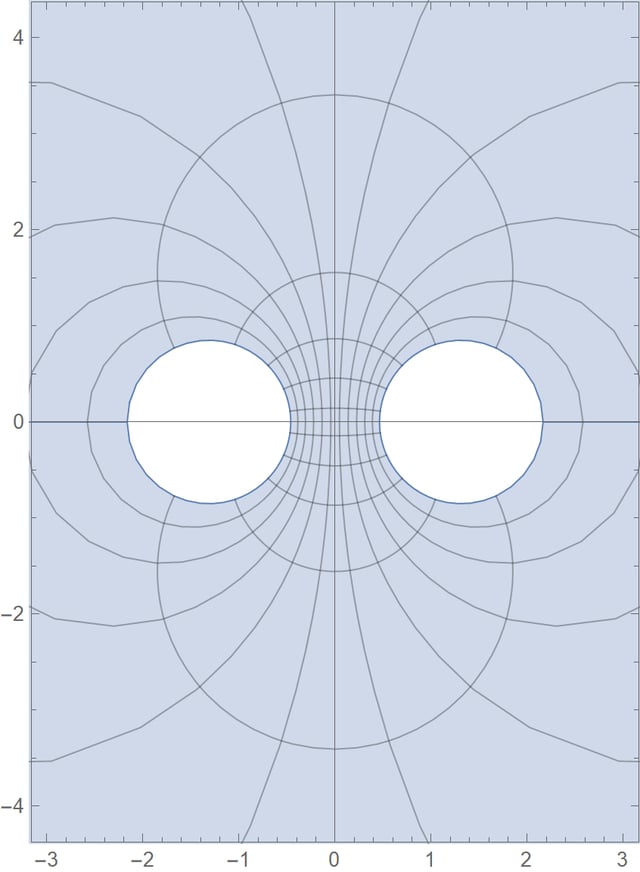
Mesh -> 20to theParametricPlot. $\endgroup$