7
$\begingroup$

I am trying to solve the heat equation for a system made of a cylinder (hot) that is suddenly immersed in a cooling medium (cold). I am doing this using a 1D approximation with single differential equation (in cylindrical coordinates) and physical properties that vary in space. The code is:

diamcyl = 0.800;
T1 = 140;
T2 = -20;

k2 = 0.58;    (* W/mK *)
rho2 = 1000;   (* kg/m3 *)
Cp2 = 4200;  (* J/KgK *)

k1 = 0.128; (*W/(mK)*)
rho1 = 800; (* kg/m3 *)
Cp1 = 1670; (*J/(KgK)*)

(*properties as a function of space*)
rho[x_] := (rho1 + (rho2 - rho1)* UnitStep[x - diamcyl/2]);
k[x_] := 10^6*(k1 + (k2 - k1)* UnitStep[x - diamcyl/2]);    
Cp[x_] := (Cp1 + (Cp2 - Cp1)* UnitStep[x - diamcyl/2]);

heateq = 1/x*D[x*k[x]*D[u[x, t], x], x] == rho[x]*Cp[x]*D[u[x, t], t];

u0[x_] := (T1 + (T2 - T1)*UnitStep[x - diamcyl/2]);
solm20 = First[
   NDSolve[{heateq, u[x, 0] == u0[x], 
     u[10, t] == T2, (D[u[x, t], x] /. x -> 0.001) == 0}, 
    u, {x, 0.001, 2}, {t, 0, 5},
    Method -> {"MethodOfLines", 
      "SpatialDiscretization" -> {"TensorProductGrid", 
        "MaxPoints" -> 1000}}]];

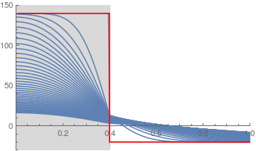
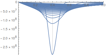
The solution transient temperature profile that I obtain looks smooth and is continuous over the boundary of the cylinder. However, the heat flux exhibits a discontinuity over this boundary.

Show[Table[
  Plot[u[x, t] /. solm20, {x, 0.001, 2}, 
   PlotRange -> {{0, 1}, {T2, T1}}, PlotRangePadding -> {None, 10}, 
   Prolog -> {LightGray, Rectangle[{0, -100}, {diamcyl/2, 200}]}, 
   GridLines -> {{diamcyl/2}, {T2}}, 
   FrameLabel -> {"distance [mm]", "temperature [\[Degree]C]"}], {t, 
   0, 2, 0.05}],

 Plot[u0[x], {x, 0.01, 2}, PlotRange -> All, Exclusions -> None, 
  PlotStyle -> Red]]

Show[Table[
  Plot[Evaluate[k[x]*D[u[x, t], x] /. solm20], {x, 0.01, 2}, 
   PlotRange -> {{0, 1}, All}, PlotRangePadding -> {None, 10}, 
   GridLines -> {{diamcyl/2}, {T2}}, 
   FrameLabel -> {"distance [mm]", "temperature [\[Degree]C]"}], {t, 
   0.01, 2, 0.05}]]

How to obtain a solution with continuous heat flux? Or, I could also ask it in this way: how to impose a Neumann condition over the boundary of the cylinder?

$\endgroup$
3
  • $\begingroup$ You have u[10, t] == T2 but at the same time {x, 0.001, 2} do you mean u[2, t] == T2? $\endgroup$
    – user21
    Commented Sep 12, 2016 at 22:42
  • $\begingroup$ Luigi, you've already asked 5 questions in this site (and 1 question in meta about how to format your code), please learn to format your code properly. If you have difficulty in understanding the answers you got in meta, just continue to ask in the comment. $\endgroup$
    – xzczd
    Commented Sep 13, 2016 at 3:36
  • $\begingroup$ sorry for the improper formatting. $\endgroup$
    – Luigi
    Commented Sep 13, 2016 at 7:31

1 Answer 1

11
$\begingroup$

Here is a way to do it:

T1 = 140;
T2 = -20;
k1 = 10^6*0.128*x;
rho1 = 800;
Cp1 = 1670;
k2 = 10^6*0.58*x;
rho2 = 1000;
Cp2 = 4200;
tend = 1/2;
lend = 2;
lm = 0.4;

v1 = rho1*Cp1;
v2 = rho2*Cp2;

opts = Method -> {"MethodOfLines", 
    "SpatialDiscretization" -> {"FiniteElement", 
      "MeshOptions" -> {"MaxCellMeasure" -> 0.01}}};

u0[x_] := Evaluate[With[{p = lm, T1 = T1, T2 = T2}, If[x < p, T1, T2]]]
(*Plot[u0[x],{x,0,lend}]*)


C1[x_] := Evaluate[With[{p = lm, k1 = k1, k2 = k2}, If[x < p, k1, k2]]]
M1[x_] := Evaluate[With[{p = lm, v1 = v1, v2 = v2}, If[x < p, v1, v2]]]

(* this depends a bit what you want *)
(*heateq1=M1[x]*D[u[x,t],t]\[Equal]1/x*Inactive[Div][{{C1[x]}}.\
Inactive[Grad][u[x,t],{x}],{x}]*)

heateq1 = 
  M1[x]*D[u[x, t], t] == 1/x*Div[{{C1[x]}}.Grad[u[x, t], {x}], {x}];

sol1 = NDSolveValue[{heateq1, u[x, 0] == u0[x]}, 
   u, {x, 0, lend}, {t, 0, tend}, opts];
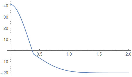
Plot[sol1[x, tend], {x, 0, lend}]

enter image description here

NIntegrate[sol1[x, tend], {x} \[Element] sol1["ElementMesh"]]
-17.231627750587393`

dsolm1 = C1[x]*D[sol1[x, t], x];
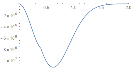
Plot[Evaluate[dsolm1 /. t -> tend], {x, 0, lend}]

enter image description here

Because there was some discussion in the comments I verified this result with another FEM tool and for the FEM I get the same results (up to some numerical acceptable difference) there. Note that the difference to the old answer is partially due to the use of the activated PDE - but that depends a bit on what you actually want to model.

Old Answer

I am not exactly sure what you are looking for, perhaps this:

heateq2 = 
  If[x < diamcyl/2, rho1*Cp1, rho2*Cp2]*D[u[x, t], t] == 
   1/x*Inactive[
      Div][{{If[x < diamcyl/2, 10^6*x*k1, 10^6*x*k2]}}.Inactive[Grad][
       u[x, t], {x}], {x}];
(*heateq2 = heateq2//Activate *)
solm20 = First[
   NDSolve[{heateq2, u[x, 0] == If[x < diamcyl/2, T1, T2](*,u[2,
     t]\[Equal]T2*)}, u, {x, 0, 2}, {t, 0, 5}, 
    Method -> {"MethodOfLines", 
      "SpatialDiscretization" -> {"FiniteElement", 
        "MeshOptions" -> {"MaxCellMeasure" -> 0.01}}}]];

Note that I set no boundary condition on the right hand side - with the finite element method that implies a Neumann zero boundary condition.

Show[Table[
  Plot[u[x, t] /. solm20, {x, 0.001, 2}, 
   PlotRange -> {{0, 1}, {T2, T1}}, PlotRangePadding -> {None, 10}, 
   Prolog -> {LightGray, Rectangle[{0, -100}, {diamcyl/2, 200}]}, 
   GridLines -> {{diamcyl/2}, {T2}}, 
   FrameLabel -> {"distance [mm]", "temperature [\[Degree]C]"}], {t, 
   0, 2, 0.05}], 
 Plot[u0[x], {x, 0.01, 2}, PlotRange -> All, Exclusions -> None, 
  PlotStyle -> Red]]

Show[Table[
  Plot[Evaluate[k[x]*D[u[x, t], x] /. solm20], {x, 0.01, 2}, 
   PlotRange -> {{0, 1}, All}, PlotRangePadding -> {None, 10}, 
   GridLines -> {{diamcyl/2}, {T2}}, 
   FrameLabel -> {"distance [mm]", "temperature [\[Degree]C]"}], {t, 
   0.01, 2, 0.05}]]

enter image description here

enter image description here

I also changed the left and side region to go from 0 and not 0.001 (this will need V11, else you can change it back to 0.001)

One thing to think about is if you want the equations to be activated, and I think you do. I tried to verify this with another FEM tool and it gives essentially the same results.

$\endgroup$
20
  • $\begingroup$ Interesting, but NDSolve will output a solution that is 1st order continuous in x-direction by default (see here for more information), why it finds a heat flux continuity solution in this case? What's the key point here? $\endgroup$
    – xzczd
    Commented Sep 13, 2016 at 2:58
  • $\begingroup$ @user21: when I run your code in Mathematica 10.0 I get the following error: NDSolve::femcnmd: The PDE coefficient {{-(If[x<0.4,10^6 x k1,10^6 x k2]/x)}} does not evaluate to a numeric matrix of dimensions {1,1}. >> $\endgroup$
    – Luigi
    Commented Sep 13, 2016 at 7:57
  • $\begingroup$ @user21: have you left out the symmetry condition (D[u[x, t], x] /. x -> 0.001) == 0 (cylinder axis) on purpose? $\endgroup$
    – Luigi
    Commented Sep 13, 2016 at 9:43
  • $\begingroup$ @xzczd, I am not exactly sure what you are referring to but I think what you mean is due to the FEM. $\endgroup$
    – user21
    Commented Sep 14, 2016 at 15:09
  • $\begingroup$ @Luigi, your first point - that's why I put the V11 stuff in the answer. The second point: in FEM if you do not specify anything that naturally means Neumann zero. See the reference for NeumannValue $\endgroup$
    – user21
    Commented Sep 14, 2016 at 15:11

Your Answer

By clicking “Post Your Answer”, you agree to our terms of service and acknowledge you have read our privacy policy.

Not the answer you're looking for? Browse other questions tagged or ask your own question.