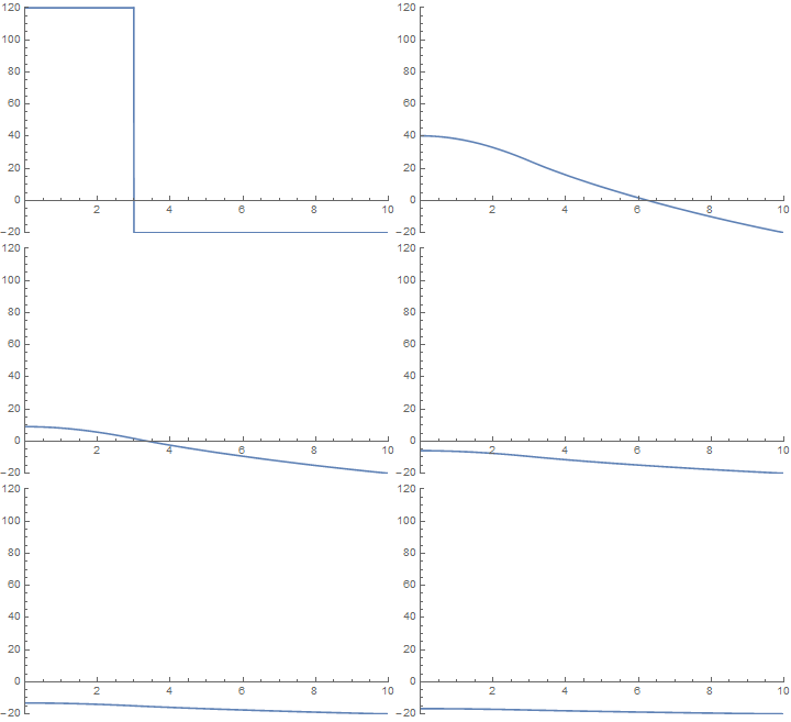
5
$\begingroup$

I am trying to simulate the temperature profile inside a very long cylinder that is suddenly immersed into a cooling fluid:

For this, I am writing a single heat equation where the physical properties are varying in space. As BC, I am assuming that I know the initial temperature profile and that I know the temperature of the cooling medium far away from the cylinder. Assuming that the radius of the cylinder is 3:

d[x_] := (1 + 4 UnitStep[x-3])
f0[x_] := (120 - 140 UnitStep[x - 3])

heateq = D[u[x, t], x, x] + 1/x*D[u[x, t], x] == 
   1/d[x]* D[u[x, t], t];

sol = First[NDSolve[{
     heateq,
     u[x, 0] == f0[x],
     u[10, t] == -20,
     (D[u[x, t], x] /. x -> 0) == 0
     },
    u[x, t], {x, 0, 10}, {t, 0, 10.}]];

frames = Table[
   Plot[Evaluate[u[x, t] /. sol], {x, 0, 10}, 
    PlotRange -> {0, 10}], {t, .001, 10, .2}];

ListAnimate[Show[#, Graphics[Line[{{5, 0}, {5, 300}}]]] & /@ frames]

However, this does not work and gives me errors such as "Infinite expression 1/0. encountered. >>".

$\endgroup$
2
  • $\begingroup$ How to solve it? $\endgroup$
    – Luigi
    Commented Aug 31, 2016 at 8:42
  • $\begingroup$ after realizing that it is sufficient not to calculate the solution at x=0, another problem becomes clear: NDSolve produces solutions that give a heat flux discontinuos over the bounday cylinder-cooling medium. Thermal conductivities are: k=0.58 W/(mK) for the cooling medium 0.21 W/(mK) for the cylinder. I am looking for heat flux continuity over the boundary. How to get it? $\endgroup$
    – Luigi
    Commented Sep 8, 2016 at 21:03

2 Answers 2

2
$\begingroup$

Here is a solution that works :

xmin = 0.1;
myMaxPoints = 500;
d[x_] := (1 + 4 UnitStep[x - 3])
f0[x_] := (120 - 140 UnitStep[x - 3])

heateq = D[u[x, t], x, x] + 1/x*D[u[x, t], x] == 1/d[x]*D[u[x, t], t];

sol = First[NDSolve[
    {heateq, u[x, 0] == f0[x], 
     u[10, t] == -20, (D[u[x, t], x] /. x -> xmin) == 0},
    u[x, t],
    {x, xmin, 10}, {t, 0, 10.},
    Method -> {"MethodOfLines", 
      "SpatialDiscretization" -> {"TensorProductGrid", 
        "MaxPoints" -> myMaxPoints}}]];

frames = Table[
   Plot[Evaluate[u[x, t] /. sol], {x, xmin, 10}, 
    PlotRange -> {{0, 10}, {-20, 120}}], {t, .001, 10, .2}];

ListAnimate[Show[#, Graphics[Line[{{5, 0}, {5, 300}}]]] & /@ frames]

enter image description here

Trial and error path to find the above solution :

  1. The initial code gives the error message :

enter image description here

This is inherent to the fact that you use polar coordinates. A solution is to make run x from 0.1 to 10. With the Neumann boundary condition : flux = 0, this is equivalent to make a small hole of diameter 0.1 in the middle of the cylinder. Physically it is totally realistic :

xmin = 0.1;
d[x_] := (1 + 4 UnitStep[x - 3])
f0[x_] := (120 - 140 UnitStep[x - 3])

heateq = D[u[x, t], x, x] + 1/x*D[u[x, t], x] == 1/d[x]*D[u[x, t], t];

sol = First[NDSolve[
    {heateq, u[x, 0] == f0[x], 
     u[10, t] == -20, (D[u[x, t], x] /. x -> xmin) == 0},
    u[x, t],
    {x, xmin, 10}, {t, 0, 10.}]];  
  1. Then we have the message :

enter image description here

This is more complicated to interpret. One has to know that :

  • MaxPoints concerns the spatial grid
  • The spatial grid is determined by the initial condition, here f0[]
  • MinStepSize is no more than "spatial length of the simulation"/MaxPoints. It exists just for convenience
  • 10000 points is clearly too much. The responsible is f0 which contains the too much stiff UnitStep function : the spatial discretization process try to much to approximate it.

There are 2 solutions :

  • replace f0[x] with something less stiff, for example 50 - 140/Pi ArcTan[100. (x - 3)]
  • or use a smaller value than default for MaxPoints. It is what we are going to do. There is a stupid difficulty : one must know that the syntax is Method -> {"MethodOfLines", "SpatialDiscretization" -> {"TensorProductGrid","MaxPoints" -> myMaxPoints}}. That is to say one has to know that MaxPoints belongs to the options of "MethodOfLines"/"TensorProductGrid" (not "FiniteElement"). And fortunately, thanks to the message that talks about MaxPoints we know that NDSolve has automatically selected the method "MethodOfLines"/"TensorProductGrid".

We can try "MaxPoints"-> 300 (more or less randomly) :

xmin = 0.1;
myMaxPoints = 300;
d[x_] := (1 + 4 UnitStep[x - 3])
f0[x_] := (120 - 140 UnitStep[x - 3])

heateq = D[u[x, t], x, x] + 1/x*D[u[x, t], x] == 1/d[x]*D[u[x, t], t];

sol = First[NDSolve[
    {heateq, u[x, 0] == f0[x], 
     u[10, t] == -20, (D[u[x, t], x] /. x -> xmin) == 0},
    u[x, t],
    {x, xmin, 10}, {t, 0, 10.},
    Method -> {"MethodOfLines", 
      "SpatialDiscretization" -> {"TensorProductGrid", 
        "MaxPoints" -> myMaxPoints}}]];  

then :

enter image description here

300 was to small. Then maybe "MaxPoints"-> 500 :

xmin = 0.1;
myMaxPoints = 500;
d[x_] := (1 + 4 UnitStep[x - 3])
f0[x_] := (120 - 140 UnitStep[x - 3])

heateq = D[u[x, t], x, x] + 1/x*D[u[x, t], x] == 1/d[x]*D[u[x, t], t];
sol = First[NDSolve[
    {heateq, u[x, 0] == f0[x], 
     u[10, t] == -20, (D[u[x, t], x] /. x -> xmin) == 0},
    u[x, t],
    {x, xmin, 10}, {t, 0, 10.},
    Method -> {"MethodOfLines", 
      "SpatialDiscretization" -> {"TensorProductGrid", 
        "MaxPoints" -> myMaxPoints}}]];

That OK, no more warning.

Then, only at end, we can try make the animation :

frames = Table[
   Plot[Evaluate[u[x, t] /. sol], {x, xmin, 10}, 
    PlotRange -> {{0, 10}, {-20, 120}}], {t, .001, 10, .2}];
ListAnimate[Show[#, Graphics[Line[{{5, 0}, {5, 300}}]]] & /@ frames]
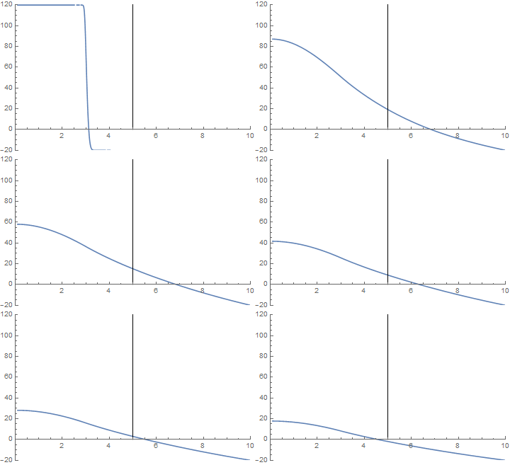
Note : The step in the diffusivity coefficient d[x] is not very visible. It seems to be normal, though I have not investigated a lot.

$\endgroup$
4
  • $\begingroup$ "The step in the diffusivity coefficient d[x] is not very visible." Actually d[x] won't cause any visible step in the solution, because in this case NDSolve automatically finds a solution that is 1st order continuous in x-direction. (For more information you may want to read this: mathematica.stackexchange.com/a/121739/1871). OP doesn't mention if (s)he wants a solution that is heat flux continuous, but if (s)he really wants one, (s)he should show us the thermal conductivities of cooling medium and cylinder. (d[x] is just thermal diffusivity.) $\endgroup$
    – xzczd
    Commented Sep 7, 2016 at 3:33
  • $\begingroup$ thermal conductivities are k=0.58 W/(mK) for the cooling medium and 0.21 W/(mK) for the cylinder. I am looking for heat flux continuity over the boundary. $\endgroup$
    – Luigi
    Commented Sep 7, 2016 at 8:08
  • $\begingroup$ and my code will give me a heat flux that is discontinuos over the bounday cylinder-cooling medium k[x_] := (0.21 + (0.58 - 0.21))* UnitStep[x - 3] Plot[k[x]*D[u[x, t], t] /. t -> 0.5 /. sol, {x, 0.1, 2}, PlotRange -> {{0, 2}, All}, FrameLabel -> {"distance", "heat flux"}] so the question becomes: how to write a boundary condition that leads to a solution with continuous heat flux? $\endgroup$
    – Luigi
    Commented Sep 7, 2016 at 9:15
  • $\begingroup$ @Luigi You should add this to your question. $\endgroup$
    – xzczd
    Commented Sep 8, 2016 at 11:11
2
$\begingroup$

Just avoid evaluating when x=0

sol = NDSolve[{
   (D[u[t, x], x, x] + (1/x) D[u[t, x], x]) - (1/d[x]) D[u[t, x],t] ==
    NeumannValue[0, x == 0.001],
   u[0, x] == f0[x],
   u[t, 10] == -20}, u, {t, 0, 30}, {x, 0.001, 10}, 
  Method -> {"MethodOfLines", "TemporalVariable" -> t, 
  "SpatialDiscretization" -> {"FiniteElement", 
  "MeshOptions" -> {"MaxCellMeasure" -> {"Length" -> 0.01}}}}]

frames = Table[
   Plot[Evaluate[u[t, x] /. sol], {x, 0, 10}, 
    PlotRange -> {{0, 10}, {-20, 120}}], {t, 0, 30, 1}];

ListAnimate[Show[#, Graphics[Line[{{3, 0}, {3, 300}}]]] & /@ frames]

enter image description here

$\endgroup$
1
  • $\begingroup$ The parentheses aren't necessary. (1/x) D[u[t, x], x] == 1/x D[u[t, x], x] returns True :) $\endgroup$
    – xzczd
    Commented Sep 6, 2016 at 14:50

Your Answer

By clicking “Post Your Answer”, you agree to our terms of service and acknowledge you have read our privacy policy.

Not the answer you're looking for? Browse other questions tagged or ask your own question.