Return to Answer

I am not exactly sure what you are looking for, perhaps this:

Here is a way to do it:

T1 = 140;
T2 = -20;
k1 = 10^6*0.128*x;
rho1 = 800;
Cp1 = 1670;
k2 = 10^6*0.58*x;
rho2 = 1000;
Cp2 = 4200;
tend = 1/2;
lend = 2;
lm = 0.4;

v1 = rho1*Cp1;
v2 = rho2*Cp2;

opts = Method -> {"MethodOfLines", 
    "SpatialDiscretization" -> {"FiniteElement", 
      "MeshOptions" -> {"MaxCellMeasure" -> 0.01}}};

u0[x_] := Evaluate[With[{p = lm, T1 = T1, T2 = T2}, If[x < p, T1, T2]]]
(*Plot[u0[x],{x,0,lend}]*)


C1[x_] := Evaluate[With[{p = lm, k1 = k1, k2 = k2}, If[x < p, k1, k2]]]
M1[x_] := Evaluate[With[{p = lm, v1 = v1, v2 = v2}, If[x < p, v1, v2]]]

(* this depends a bit what you want *)
(*heateq1=M1[x]*D[u[x,t],t]\[Equal]1/x*Inactive[Div][{{C1[x]}}.\
Inactive[Grad][u[x,t],{x}],{x}]*)

heateq1 = 
  M1[x]*D[u[x, t], t] == 1/x*Div[{{C1[x]}}.Grad[u[x, t], {x}], {x}];

sol1 = NDSolveValue[{heateq1, u[x, 0] == u0[x]}, 
   u, {x, 0, lend}, {t, 0, tend}, opts];
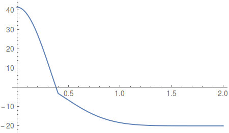
Plot[sol1[x, tend], {x, 0, lend}]

NIntegrate[sol1[x, tend], {x} \[Element] sol1["ElementMesh"]]
-17.231627750587393`

dsolm1 = C1[x]*D[sol1[x, t], x];
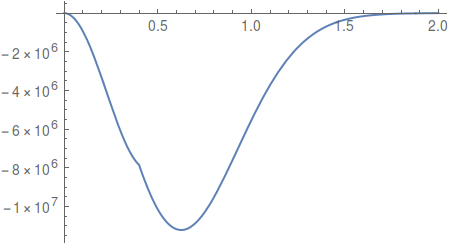
Plot[Evaluate[dsolm1 /. t -> tend], {x, 0, lend}]

Because there was some discussion in the comments I verified this result with another FEM tool and for the FEM I get the same results (up to some numerical acceptable difference) there. Note that the difference to the old answer is partially due to the use of the activated PDE - but that depends a bit on what you actually want to model.

Old Answer

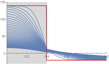
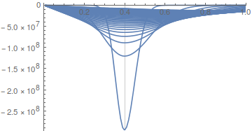
I am not exactly sure what you are looking for, perhaps this:

heateq2 = 
  If[x < diamcyl/2, rho1*Cp1, rho2*Cp2]*D[u[x, t], t] == 
   1/x*Inactive[
      Div][{{If[x < diamcyl/2, 10^6*x*k1, 10^6*x*k2]}}.Inactive[Grad][
       u[x, t], {x}], {x}];
solm20 = First[
   NDSolve[{heateq2, u[x, 0] == If[x < diamcyl/2, T1, T2](*,u[2,
     t]\[Equal]T2*)}, u, {x, 0, 2}, {t, 0, 5}, 
    Method -> {"MethodOfLines", 
      "SpatialDiscretization" -> {"FiniteElement", 
        "MeshOptions" -> {"MaxCellMeasure" -> 0.01}}}]];

I also changed the left and side region to go from 0 and not 0.001 (this will need V11, else you can change it back to 0.001)

Update:

As pointed out by @xzczd in the comments you could also use:

heateq2 = (*If[x < diamcyl/2, rho1*Cp1, rho2*Cp2]**)D[u[x, t], t] == 1/x*Inactive[ Div][{{If[x < diamcyl/2, 10^6*x*k1/(rho1*Cp1), 10^6*x*k2/(rho2*Cp2)]}}.Inactive[Grad][ u[x, t], {x}], {x}];

Which gives:

heateq2 = 
  If[x < diamcyl/2, rho1*Cp1, rho2*Cp2]*D[u[x, t], t] == 
   1/x*Inactive[
      Div][{{If[x < diamcyl/2, 10^6*x*k1, 10^6*x*k2]}}.Inactive[Grad][
       u[x, t], {x}], {x}];
(*heateq2 = heateq2//Activate *)
solm20 = First[
   NDSolve[{heateq2, u[x, 0] == If[x < diamcyl/2, T1, T2](*,u[2,
     t]\[Equal]T2*)}, u, {x, 0, 2}, {t, 0, 5}, 
    Method -> {"MethodOfLines", 
      "SpatialDiscretization" -> {"FiniteElement", 
        "MeshOptions" -> {"MaxCellMeasure" -> 0.01}}}]];

I also changed the left and side region to go from 0 and not 0.001 (this will need V11, else you can change it back to 0.001)

One thing to think about is if you want the equations to be activated, and I think you do. I tried to verify this with another FEM tool and it gives essentially the same results.

I am not exactly sure what you are looking for, perhaps this:

heateq2 = 
  If[x < diamcyl/2, rho1*Cp1, rho2*Cp2]*D[u[x, t], t] == 
   1/x*Inactive[
      Div][{{If[x < diamcyl/2, 10^6*x*k1, 10^6*x*k2]}}.Inactive[Grad][
       u[x, t], {x}], {x}];
solm20 = First[
   NDSolve[{heateq2, u[x, 0] == If[x < diamcyl/2, T1, T2](*,u[2,
     t]\[Equal]T2*)}, u, {x, 0, 2}, {t, 0, 5}, 
    Method -> {"MethodOfLines", 
      "SpatialDiscretization" -> {"FiniteElement", 
        "MeshOptions" -> {"MaxCellMeasure" -> 0.01}}}]];

Note that I set no boundary condition on the right hand side - with the finite element method that implies a Neumann zero boundary condition.

Show[Table[
  Plot[u[x, t] /. solm20, {x, 0.001, 2}, 
   PlotRange -> {{0, 1}, {T2, T1}}, PlotRangePadding -> {None, 10}, 
   Prolog -> {LightGray, Rectangle[{0, -100}, {diamcyl/2, 200}]}, 
   GridLines -> {{diamcyl/2}, {T2}}, 
   FrameLabel -> {"distance [mm]", "temperature [\[Degree]C]"}], {t, 
   0, 2, 0.05}], 
 Plot[u0[x], {x, 0.01, 2}, PlotRange -> All, Exclusions -> None, 
  PlotStyle -> Red]]

Show[Table[
  Plot[Evaluate[k[x]*D[u[x, t], x] /. solm20], {x, 0.01, 2}, 
   PlotRange -> {{0, 1}, All}, PlotRangePadding -> {None, 10}, 
   GridLines -> {{diamcyl/2}, {T2}}, 
   FrameLabel -> {"distance [mm]", "temperature [\[Degree]C]"}], {t, 
   0.01, 2, 0.05}]]

I also changed the left and side region to go from 0 and not 0.001 (this will need V11, else you can change it back to 0.001)

I am not exactly sure what you are looking for, perhaps this:

heateq2 = 
  If[x < diamcyl/2, rho1*Cp1, rho2*Cp2]*D[u[x, t], t] == 
   1/x*Inactive[
      Div][{{If[x < diamcyl/2, 10^6*x*k1, 10^6*x*k2]}}.Inactive[Grad][
       u[x, t], {x}], {x}];
solm20 = First[
   NDSolve[{heateq2, u[x, 0] == If[x < diamcyl/2, T1, T2](*,u[2,
     t]\[Equal]T2*)}, u, {x, 0, 2}, {t, 0, 5}, 
    Method -> {"MethodOfLines", 
      "SpatialDiscretization" -> {"FiniteElement", 
        "MeshOptions" -> {"MaxCellMeasure" -> 0.01}}}]];

Note that I set no boundary condition on the right hand side - with the finite element method that implies a Neumann zero boundary condition.

Show[Table[
  Plot[u[x, t] /. solm20, {x, 0.001, 2}, 
   PlotRange -> {{0, 1}, {T2, T1}}, PlotRangePadding -> {None, 10}, 
   Prolog -> {LightGray, Rectangle[{0, -100}, {diamcyl/2, 200}]}, 
   GridLines -> {{diamcyl/2}, {T2}}, 
   FrameLabel -> {"distance [mm]", "temperature [\[Degree]C]"}], {t, 
   0, 2, 0.05}], 
 Plot[u0[x], {x, 0.01, 2}, PlotRange -> All, Exclusions -> None, 
  PlotStyle -> Red]]

Show[Table[
  Plot[Evaluate[k[x]*D[u[x, t], x] /. solm20], {x, 0.01, 2}, 
   PlotRange -> {{0, 1}, All}, PlotRangePadding -> {None, 10}, 
   GridLines -> {{diamcyl/2}, {T2}}, 
   FrameLabel -> {"distance [mm]", "temperature [\[Degree]C]"}], {t, 
   0.01, 2, 0.05}]]

I also changed the left and side region to go from 0 and not 0.001 (this will need V11, else you can change it back to 0.001)

Update:

As pointed out by @xzczd in the comments you could also use:

heateq2 = (*If[x < diamcyl/2, rho1*Cp1, rho2*Cp2]**)D[u[x, t], t] == 1/x*Inactive[ Div][{{If[x < diamcyl/2, 10^6*x*k1/(rho1*Cp1), 10^6*x*k2/(rho2*Cp2)]}}.Inactive[Grad][ u[x, t], {x}], {x}];

Which gives: