Remove noise from data

Question

Hi, as you can see above I have some experimental data which has a large offset and shows clear noise fluctations around the tendency of the curve. I wanted to ask if someone could suggest me a method to remove the noise, withoud eliminating the oscillations.

Using EstimateBackground[] I was able to envelope the oscillations (yellow and green curves) but as you can see, the noise spikes make it very uncertain. The red curve was my attempt to reproduce the tendency of the oscillations and smoothing the data, using a median noise filter (Median noise filter), but it is a little off.

Thanks for your help!

data = Uncompress[FromCharacterCode[
  Flatten[ImageData[Import["https://i.sstatic.net/7agjd.png"],"Byte"]]]]

Answer 1

You could try BilateralFilter:

ListLinePlot[{data, 
  BilateralFilter[data, 2, .5, MaxIterations -> 25]}, 
 PlotStyle -> {Thin, Red}]

Or alternatively, MeanShiftFilter can produce similar results:

ListLinePlot[{data, 
  MeanShiftFilter[data, 5, .5, MaxIterations -> 10]}, 
 PlotStyle -> {Thin, Red}]

Third alternative, as mentioned by @Xavier in the comments, is to apply TrimmedMean over a sliding window:

ListLinePlot[{data, ArrayFilter[TrimmedMean, data, 20]}, 
 PlotStyle -> {Thin, Red}]

As requested in the comments, a Savitzky Golay filter:

ListLinePlot[{
  data,
  ListConvolve[SavitzkyGolayMatrix[{10}, 2], 
   ArrayPad[data, 10, "Fixed"]]
  }, PlotStyle -> {Thin, Red}]

For comparison:

Show[
 ListPlot[data, PlotLegends -> {"Raw Data"}],
 ListLinePlot[{BilateralFilter[data, 2, .5, MaxIterations -> 25], 
   MeanShiftFilter[data, 5, .5, MaxIterations -> 10], 
   ArrayFilter[TrimmedMean, data, 20], 
   ListConvolve[SavitzkyGolayMatrix[{10}, 2], 
    ArrayPad[data, 10, "Fixed"]]},
  PlotLegends -> {"BilateralFilter", "MeanShiftFilter", 
    "ArrayFilter[TrimmedMean]", "SavitzkyGolay"}], ImageSize -> 800]

• MeanShiftFilter and BilateralFilter produce a smooth result, and are almost indistinguishable with these parameters.
• The sliding window TrimmedMean filter technique looks more "ragged" in comparison.
• I couldn't get a smooth curve with the Savitzky Golay filter, probably because the large outliers aren't well suited to linear filtering.

You'll have to play with the parameters to each of them to get the results you want.

Answer 2

I would suggest using a median filter with small radius to eliminate the large spikes, then a mean filter to smooth the remaining signal. @Xavier essentially combines these two filters by using TrimmedMean.

Other than the large spikes, your data seem to have a strong signal with a period of about 10 points. You could use BandstopFilter to remove this, or LowpassFilter to eliminate this oscillation plus higher frequencies.

In the following, I removed the mean from your original data.

Manipulate[
   Module[{f},
      f = LowpassFilter[MedianFilter[data, r], w];
      ListLinePlot[{data, f - Mean[f]}, ImageSize -> 600, Frame -> True, 
                   PlotStyle -> {Thin, Thick}]
   ],
   {{r, 0, "Median Filter Radius"}, 0, 10, 1, Appearance -> "Labeled"},
   {{w, 3., "Cutoff Angular Frequency"}, 0.002,Pi, Appearance -> "Labeled"}]

Answer 3

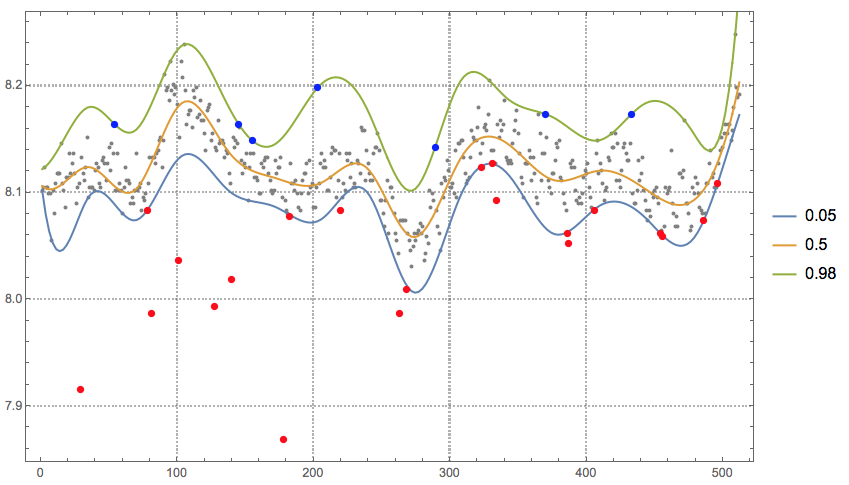
I am not sure what is called "noise" in the question, from the description, I think it is about removing outliers. This solution uses Quantile regression twice: to detect the outliers, and then to find quantile regression curves in the data without the outliers.

Load the package:

Import["https://raw.githubusercontent.com/antononcube/MathematicaForPrediction/master/QuantileRegression.m"]

Adding x-coordinates to the data:

data = Transpose[{Range[Length[data]], data}];

Selection of quantiles to detect the outliers:

qs = {0.05, 0.5, 0.98};
{qs[[1]], 1 - qs[[-1]]}*Length[data]
(* {25.6, 10.24} *)

Quantile regression with the selected quantiles:

qfuncs = QuantileRegression[data, 15, qs];

Finding the top outliers:

topOutliers = Select[data, qfuncs[[-1]][#[[1]]] < #[[2]] &]

(* {{54, 8.16422}, {145, 8.16422}, {155, 8.14875}, {203, 
  8.19841}, {289, 8.14254}, {370, 8.17358}, {433, 8.17358}} *)

Finding the bottom outliers:

bottomOutliers = Select[data, qfuncs[[1]][#[[1]]] > #[[2]] &]

(* {{29, 7.9156}, {78, 8.08349}, {81, 7.98714}, {101, 
  8.03685}, {127, 7.99335}, {140, 8.01821}, {178, 7.8689}, {182, 
  8.07728}, {220, 8.08349}, {263, 7.98714}, {268, 8.00884}, {323, 
  8.12381}, {331, 8.12696}, {334, 8.09276}, {386, 8.0617}, {387, 
  8.05243}, {406, 8.08349}, {454, 8.0617}, {456, 8.05864}, {486, 
  8.07412}, {496, 8.10833}} *)

Plot data, regression quantiles, and outliers:

qfPlot = ListLinePlot[
   Table[{#, qfuncs[[i]][#]} & /@ 
     Rescale[Range[0, 1, 0.005], {0, 1}, MinMax[data[[All, 1]]]], {i, 
     1, Length[qfuncs]}], PerformanceGoal -> "Quality", 
   PlotRange -> All, PlotTheme -> "Detailed", PlotLegends -> qs];
Show[{ListPlot[data, PlotRange -> All, PlotStyle -> {GrayLevel[0.5]}, 
   PlotTheme -> "Detailed"], qfPlot, 
  ListPlot[{topOutliers, bottomOutliers}, PlotStyle -> {{
      Blue, PointSize[0.01]}, {Red, PointSize[0.01]}}]}, 
 ImageSize -> 600]

Remove the outliers from the data:

newData = Complement[data, Join[topOutliers, bottomOutliers]];

Make another quantile regression computation over the new data. (This time is to facilitate analysis instead of detecting outliers.)

Block[{data = newData, qfuncs, qs = {0.05, 0.25, 0.5, 0.75, 0.95}},
 qfuncs = QuantileRegression[data, 40, qs]; 
 Show[{ListPlot[data, PlotStyle -> GrayLevel[0.5], PlotRange -> All, 
    PlotTheme -> "Detailed"], 
   ListLinePlot[
    Transpose@
     Map[Thread[{#, Through[qfuncs[#]]}] &, 
      Rescale[Range[0, 1, 0.005], {0, 1}, MinMax[data[[All, 1]]]]], 
    PlotStyle -> Map[If[# == 0.5, Thick, Thin] &, qs], 
    PlotLegends -> qs]}, ImageSize -> 600]]

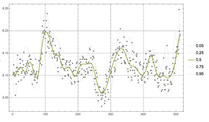
Obviously other methods of signal analysis can be applied to the cleaned data. In this particular case, the cleaned data would give better results for the conditional PDF/CDF reconstruction shown in this blog post "Estimation of conditional density distributions".