How to interpret the results of PCA

Question

There is a larger matrix (1500 rows x 40 columns), 1500 observations x 40 variables. then I follow the procedures of PCA(Principal components analysis), 1. find correlation 2. find eigenvalues 3. find Eigenvectors I have got the result (Mathematica)

dataCorrEigenvalues/Total@dataCorrEigenvalues

{0.647833, 0.128731, 0.0843738, 0.0519215, 0.0246577, 0.018331, \
0.0100494, 0.00657219, 0.0054721, 0.00373078, 0.00310175, 0.00244999, \
0.0022292, 0.00190861, 0.00166728, 0.00124446, 0.00113064, \
0.00093684, 0.000673087, 0.000579798, 0.00049716, 0.000425554, \
0.000371012, 0.000261027, 0.000225517, 0.000173631, 0.000133479, \
0.000128954, 0.000103792, 0.0000853669}

FoldList[Plus, dataCorrEigenvalues/Total@dataCorrEigenvalues]

{0.647833, 0.776564, 0.860938, 0.91286, 0.937517, 0.955848, 0.965898, \
0.97247, 0.977942, 0.981673, 0.984775, 0.987225, 0.989454, 0.991362, \
0.99303, 0.994274, 0.995405, 0.996342, 0.997015, 0.997595, 0.998092, \
0.998517, 0.998888, 0.999149, 0.999375, 0.999548, 0.999682, 0.999811, \
0.999915, 1.}

As I know the first 6 components explain about 95% of the variability, However, I don't understand how to use these components for data analysis.

The projection Matrix "w" as the following

w = dataCorrEigenvectors[[All, 1 ;; 4]];

I try to calculate the dot product of W against data, however, it seems the result is not same as expectation.

PC5 = data.w;

Please feel free to command and advise what I should do. Thank you.

Answer 1

I generated a multivariate data set to play with called fakedata (see at the bottom of the post). This contains five groups of samples, each in 25-replicate. Each sample is described by five descriptors with very different ranges (see at the bottom of the post for the generation of the data). fakedata therefore is a $125\times5$ matrix: this is smaller than yours, but these methods are obviously scalable.

First of all, as I mentioned in the comments, you should be aware of the fact that Mathematica has a built-in PrincipalComponents function

builtinscores = PrincipalComponents[fakedata, Method -> "Correlation"];

Having said that, however, trying to roll your own is simple and instructive. In addition, to the fun of doing it by hand, it also gives you access to the data you would need to construct e.g. loading plots and other interesting descriptors of the multivariate analysis.

As you mentioned, one obtains the transformation matrix by calculating the eigenvectors of the correlation matrix of the original data. In order to obtain the transformed PCA scores from the original data, you need to Standardize your data first, then dot-multiply it by those eigenvectors (check out Mathematica's definition of Eigensystem to see why we want to Transpose those eigenvectors first):

manscores = Standardize[fakedata].Transpose[Eigenvectors[Correlation[fakedata]]];

... and this is really all there is to it!

---

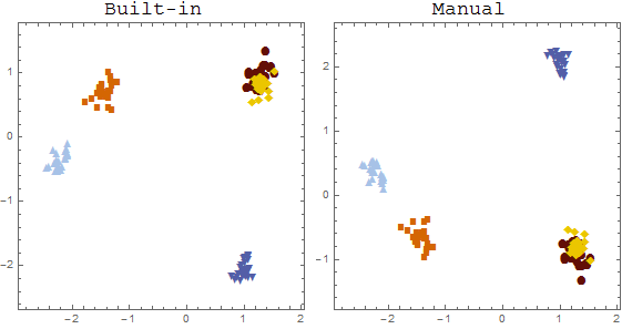
In fact, we can graphically check that we obtain the same PCA scores with the two methods. Here is a quick helper function to plot a 2D PCA score plot:

Clear[plotscores]
plotscores[scores_] := ListPlot[
   Partition[scores[[All, 1 ;; 2]], 25],
   PlotRange -> All, PlotRangePadding -> Scaled[0.1],
   PlotMarkers -> {Automatic, Medium}, PlotStyle -> ColorData[22, "ColorList"],
   AspectRatio -> 1, Frame -> True, Axes -> False, ImageSize -> Scaled[0.33]
 ]

Using this function, we can generate score plots from the scores calculated before by hand vs using the built-in function:

builtin = plotscores[builtinscores];
manual = plotscores[manscores];
Grid[{Style[#, FontSize -> 18] & /@ {"Built-in", "Manual"}, {builtin, manual}}]

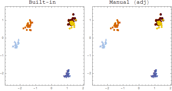
You will notice that the two plots are identical up to a sign change. Of course sign is irrelevant here, so we can adjust the sign of the ordinate of the manually calculated:

manualadj = plotscores[Cases[manscores, {x_, y_, rest__} -> {x, -y, rest}]];
Grid[{Style[#, FontSize -> 18] & /@ {"Built-in", "Manual (adj)"}, {builtin, manualadj}}]

---

As a small aside, in order to calculate percentage contributions of each principal component you can simply use:

Normalize[Eigenvalues[Correlation[fakedata]], Total]

(* Out: {0.456492, 0.261667, 0.202659, 0.0648009, 0.0143812} *)

For cumulative contributions, Accumulate is your friend, rather than using your FoldList expression:

Accumulate[%]

(* Out: {0.456492, 0.718159, 0.920818, 0.985619, 1.} *)

---

Finally, here is how I generated fakedata:

Clear[samplereplicates]
samplereplicates[mu_ /; (Dimensions[mu] == {5}), n_Integer] :=
 RandomVariate[#, n] &@
  MultinormalDistribution[
   mu,
   {{0.0001, 0., 0., 0., 0.},
    {0., 0.0004, 0., 0., 0.},
    {0., 0., 2250000, 0, 0.},
    {0., 0., 0, 5290000, 0.},
    {0., 0., 0., 0., 0.000025}}
  ]

SeedRandom[20160122]
fakedata = Join[
   samplereplicates[{0.21, 0.85, 28000, 15000, 0.185}, 25],
   samplereplicates[{0.15, 0.65, 35000, 75000, 0.185}, 25],
   samplereplicates[{0.35, 0.80, 25000, 25000, 0.185}, 25], 
   samplereplicates[{0.02, 0.50, 45000, 50000, 0.185}, 25],
   samplereplicates[{0.46, 0.70, 55000, 15000, 0.185}, 25]
 ];