Stress calculations using finite elements

Question

A standard engineering problem is to calculate stresses in a structure due to applied forces. With the inclusion of the finite element method in version 10 this question attempts to investigate how this may be done. Normal, Subscript[σ, x] Subscript[σ, y] and shear Subscript[σ, x y] stresses are calculate from displacements (in two dimensions) by

These stresses are gradients of the displacements u(x,y) and v(x,y) in the x and y directions. When these equations are combined with the equilibrium conditions

we get the differential equations for plain stress

Unfortunately these equations cannot be entered directly into NDSolveValue. I tried in this post and the ever helpful user21 showed that the way the equation is entered makes a significant difference. I feel I should be able to construct the required equation from mine but it is beyond me. A secondary question is can someone write a parser that could interpret textbook equations in the needed manner? The question here is how to best extract stresses from a finite element analysis. Also, how can one conveniently put in stresses (or forces) on the boundaries? The required version of the differential equation has been provided by user21. My first attempt is to input the above equation for stress together with the required version of the differential equation.

Needs["NDSolve`FEM`"];
 ps = {Inactive[
      Div][({{0, -((Y ν)/(1 - ν^2))}, {-((Y (1 - ν))/(
          2 (1 - ν^2))), 0}}.Inactive[Grad][v[x, y], {x, y}]), {x,
       y}] + Inactive[
      Div][({{-(Y/(1 - ν^2)), 
         0}, {0, -((Y (1 - ν))/(2 (1 - ν^2)))}}.Inactive[
         Grad][u[x, y], {x, y}]), {x, y}], 
   Inactive[
      Div][({{0, -((Y (1 - ν))/(2 (1 - ν^2)))}, {-((Y ν)/(
          1 - ν^2)), 0}}.Inactive[Grad][u[x, y], {x, y}]), {x, 
      y}] + Inactive[
      Div][({{-((Y (1 - ν))/(2 (1 - ν^2))), 
         0}, {0, -(Y/(1 - ν^2))}}.Inactive[Grad][
        v[x, y], {x, y}]), {x, y}]};

L = 1;
h = 0.125;
ss = 5; (* Shear stress on beam *)
reg = Rectangle[{0, -h}, {L, h}];
mesh = ToElementMesh[reg];
mesh["Wireframe"]

{uif, vif, σxif, σyif, σxyif} = NDSolveValue[{
     ps == {0, NeumannValue[ss, x == L]},

     σx[x, y] == 
      Y/(1 - ν^2) (D[u[x, y], x] + ν D[v[x, y], y] ),
     σy[x, y] == 
      Y/(1 - ν^2) (D[v[x, y], y] + ν D[u[x, y], x] ),
     σxy[x, y] == 
       Y/(1 - ν^2) (1 - ν)/2 (D[u[x, y], y] + D[v[x, y], x] ),

     DirichletCondition[u[x, y] == 0, x == 0],
     DirichletCondition[v[x, y] == 0, x == 0]

     } /. {Y -> 10^3, ν -> 33/100},
   {u, v, σx, σy, σxy},
   {x, y} ∈ mesh];

The displacement results are

dmesh = ElementMeshDeformation[mesh, {uif, vif}, "ScalingFactor" -> 1];
Show[{
  mesh["Wireframe"],
  dmesh["Wireframe"[
    "ElementMeshDirective" -> Directive[EdgeForm[Red], FaceForm[]]]]}]

The stress results look good

Plot3D[σxif[x, y], {x, y} ∈ mesh, 
 BoxRatios -> {4, 1, 1}, PlotRange -> All]
Plot3D[σxyif[x, y], {x, y} ∈ mesh, 
 BoxRatios -> {4, 1, 1}, PlotRange -> All]

As a check one can use the approximate results of Euler-Bernoulli beam theory which is good away from the ends where the finite element method is more correct.

Plot[{σxif[L/2, y], -((ss 12 2 h  0.5)/(2 h)^3) y }, {y, -h, 
  h}, PlotLegends -> LineLegend[{"Calculated", "Theory"}]]
Plot[{σxyif[L/2, y], 6  ss/(8 h^3) 2 h (h^2 - y^2)}, {y, -h, 
  h}, PlotLegends -> LineLegend[{"Calculated", "Theory"}]]

These results are very good.

As these equations work I was hoping that the stresses on the boundaries could be entered directly as a DirichletCondition rather than NeumannValue

{uif, vif, σxif, σyif, σxyif} = NDSolveValue[{
     ps == {0, 0},

     σx[x, y] == 
      Y/(1 - ν^2) (D[u[x, y], x] + ν D[v[x, y], y] ),
     σy[x, y] == 
      Y/(1 - ν^2) (D[v[x, y], y] + ν D[u[x, y], x] ),
     σxy[x, y] == 
       Y/(1 - ν^2) (1 - ν)/2 (D[u[x, y], y] + D[v[x, y], x] ),

     DirichletCondition[u[x, y] == 0, x == 0],
     DirichletCondition[v[x, y] == 0, x == 0],
     DirichletCondition[σxy[x, y] == ss, x == L],
     DirichletCondition[σx[x, y] == 0, x == L],
     DirichletCondition[σy[x, y] == 0, x == L]

     } /. {Y -> 10^3, ν -> 33/100},
   {u, v, σx, σy, σxy},
   {x, y} ∈ mesh];

dmesh = ElementMeshDeformation[mesh, {uif, vif}, 
   "ScalingFactor" -> 10];
Show[{
  mesh["Wireframe"],
  dmesh["Wireframe"[
    "ElementMeshDirective" -> Directive[EdgeForm[Red], FaceForm[]]]]}]

Plot3D[σxyif[x, y], {x, y} ∈ mesh, 
 BoxRatios -> {4, 1, 1}, PlotRange -> All]

However, this approach does not work. So what is the best way of putting stresses into, and getting stresses out of, the finite element method? Thanks

Answer 1

Update:

Since version 13.0, all of this has become much, much simpler:

Set up the geometry:

Needs["NDSolve`FEM`"]
L = 1;
h = 0.125;
(*Shear stress on beam*)
ss = 5;
reg = Rectangle[{0, -h}, {L, h}];
mesh = ToElementMesh[reg];

Now, we can use the solid mechanics functionality. We set up variables and parameters:

vars = {{u[x, y], v[x, y]}, {x, y}};
pars = <|"YoungModulus" -> 10^3, "PoissonRatio" -> 33/100, 
   "ModelForm" -> "PlaneStress", "Thickness" -> 1|>;

Setup an solve the equations:

displacement = 
  NDSolveValue[{SolidMechanicsPDEComponent[vars, pars] == 
     SolidBoundaryLoadValue[x == L, vars, 
      pars, <|"Pressure" -> {0, ss}|>], 
    SolidFixedCondition[x == 0, vars, pars]}, 
   vars[[1]], {x, y} \[Element] mesh];

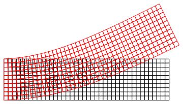
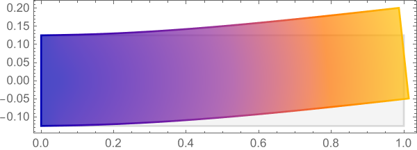
Visualize the displacement:

VectorDisplacementPlot[displacement, {x, y} \[Element] reg]

Compute strain, stress and von Mises stress:

strain = SolidMechanicsStrain[vars, pars, displacement];
stress = SolidMechanicsStress[vars, pars, strain];
vonMisesStress = PDEModels`VonMisesStress[vars, pars, stress];

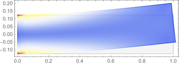
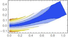
Visualize the von Mises stress on the deformed geometry:

VectorDisplacementPlot[{displacement, 
  vonMisesStress}, {x, y} \[Element] reg, 
 ColorFunction -> "TemperatureMap"]

Voilà.

Old post

There are several part to you question and I'll try to tackle them one by one (not sure I'll be able to do this in one go)

How to calculate stresses

Here is the model problem.

L = 1;
h = 0.125;
(*Shear stress on beam*)
ss = 5;
reg = Rectangle[{0, -h}, {L, h}];
mesh = ToElementMesh[reg];
materialParameters = {Y -> 10^3, \[Nu] -> 33/100};

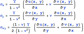
We use a plane stress formulation as you derived it and under consideration that we do not want the operator to evaluate:

Needs["NDSolve`FEM`"];
ps = {Inactive[
      Div][({{-(Y/(1 - \[Nu]^2)), 
         0}, {0, -((Y (1 - \[Nu]))/(2 (1 - \[Nu]^2)))}}.Inactive[
         Grad][u[x, y], {x, y}]), {x, y}] + 
    Inactive[
      Div][({{0, -((Y \[Nu])/(1 - \[Nu]^2))}, {-((Y (1 - \[Nu]))/(2 \
(1 - \[Nu]^2))), 0}}.Inactive[Grad][v[x, y], {x, y}]), {x, y}], 
   Inactive[
      Div][({{0, -((Y (1 - \[Nu]))/(2 (1 - \[Nu]^2)))}, {-((Y \
\[Nu])/(1 - \[Nu]^2)), 0}}.Inactive[Grad][u[x, y], {x, y}]), {x, y}] +
     Inactive[
      Div][({{-((Y (1 - \[Nu]))/(2 (1 - \[Nu]^2))), 
         0}, {0, -(Y/(1 - \[Nu]^2))}}.Inactive[Grad][
        v[x, y], {x, y}]), {x, y}]};

We then solve

{uif, vif} = 
  NDSolveValue[{ps == {0, NeumannValue[ss, x == L]}, 
     DirichletCondition[u[x, y] == 0, x == 0], 
     DirichletCondition[v[x, y] == 0, x == 0]} /. 
    materialParameters, {u, v}, {x, y} \[Element] mesh];

Note that I only included the plane stress formulation. We will recover the derivatives for the stress computation just now.

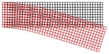
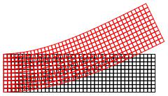
dmesh = ElementMeshDeformation[mesh, {uif, vif}, "ScalingFactor" -> 1];
Show[{mesh["Wireframe"], 
  dmesh["Wireframe"[
    "ElementMeshDirective" -> Directive[EdgeForm[Red], FaceForm[]]]]}]

Here is a function to allow to recover the derivatives:

ClearAll[VonMisesStress]
VonMisesStress[{uif_InterpolatingFunction, 
   vif_InterpolatingFunction}, fac_] := Block[
  {dd, df, mesh, coords, dv, ux, uy, vx, vy, ex, ey, gxy, sxx, syy, 
   sxy},
  dd = Outer[(D[#1[x, y], #2]) &, {uif, vif}, {x, y}];
  df = Table[Function[{x, y}, Evaluate[dd[[i, j]]]], {i, 2}, {j, 2}];
  (* the coordinates from the ElementMesh *)
  
  mesh = uif["Coordinates"][[1]];
  coords = mesh["Coordinates"];
  dv = Table[df[[i, j]] @@@ coords, {i, 2}, {j, 2}];
  
  ux = dv[[1, 1]];
  uy = dv[[1, 2]];
  vx = dv[[2, 1]];
  vy = dv[[2, 2]];
  
  ex = ux;
  ey = vy;
  gxy = (uy + vx);
  
  sxx = fac[[1, 1]]*ex + fac[[1, 2]]*ey;
  syy = fac[[2, 1]]*ex + fac[[2, 2]]*ey;
  sxy = fac[[3, 3]]*gxy;
  (*ElementMeshInterpolation[{mesh},
  Sqrt[(sxy^2) + (syy^2)+(sxx^2)]]*)
  {sxx, syy, sxy}
  ]

If you uncomment the ElementMeshInterpolation then this will compute the vonMises stress, but now it returns the stresses.

fac = Y/(1 - \[Nu]^2)*{{1, \[Nu], 0}, {\[Nu], 1, 0}, {0, 
     0, (1 - \[Nu])/2}};
facm = fac /. materialParameters;
fac // Simplify
{{Y/(1 - \[Nu]^2), (Y \[Nu])/(1 - \[Nu]^2), 0}, {(Y \[Nu])/(
  1 - \[Nu]^2), Y/(1 - \[Nu]^2), 0}, {0, 0, Y/(2 + 2 \[Nu])}}

The factor is for plane stress; it needs to be adjusted for plain strain accordingly.

(*vonMisesStress =VonMisesStress[{uif,vif},facm]*)
{sxx, syy, sxy} = 
  VonMisesStress[{uif, vif}, facm];
ifsxx = ElementMeshInterpolation[{mesh}, sxx];
ifsyy = ElementMeshInterpolation[{mesh}, syy];
ifsxy = ElementMeshInterpolation[{mesh}, sxy];

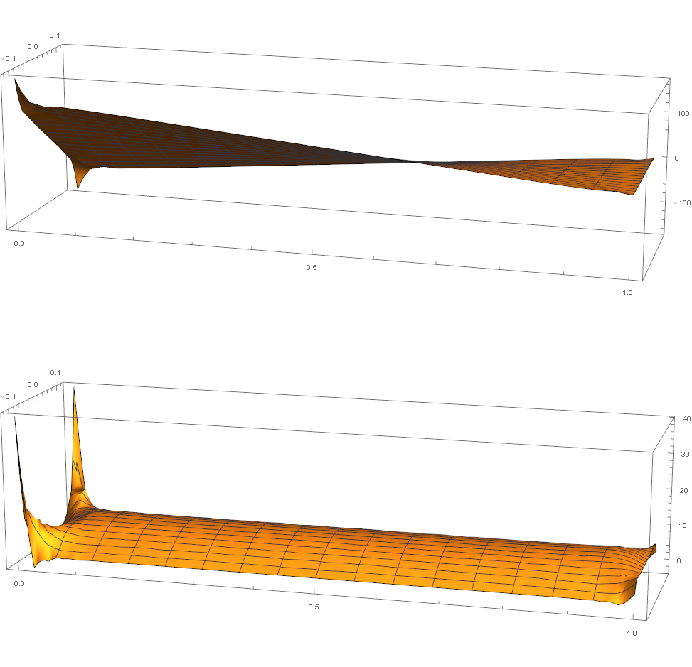
Let's compare this with your approach:

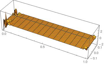
(* Plot3D[ifsxx[x, y] - \[Sigma]xif[x, y], {x, y} \[Element] mesh, 
 BoxRatios -> {4, 1, 1}, PlotRange -> All] *)
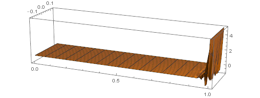
Plot3D[ifsxy[x, y] - \[Sigma]xyif[x, y], {x, y} \[Element] mesh, 
 BoxRatios -> {4, 1, 1}, PlotRange -> All]

The differences at the boundary are expected, I think. Additionally, this has the advantage of not creating additional equations that need to be solved for.

Visualize the vonMises stress in the deformed beam:

ElementMeshContourPlot[Sqrt[(sxx^2) + (syy^2) + (sxy^2)], 
 ElementMeshDeformation[uif["ElementMesh"], {uif, vif} ], 
 AspectRatio -> Automatic]

So, this is how I'd compute the stresses.

Now, let's consider some of your other questions.

How to specify forces/stresses on the region and boundary.

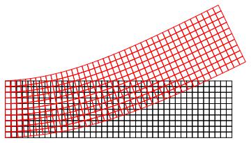
A force on the entire body (e.g. gravity)

{uif, vif} = 
  NDSolveValue[{ps == {0, -9.8}, 
     DirichletCondition[u[x, y] == 0, x == 0], 
     DirichletCondition[v[x, y] == 0, x == 0]} /. 
    materialParameters, {u, v}, {x, y} \[Element] mesh];
dmesh = ElementMeshDeformation[mesh, {uif, vif}, "ScalingFactor" -> 1];
Show[{mesh["Wireframe"], 
  dmesh["Wireframe"[
    "ElementMeshDirective" -> Directive[EdgeForm[Red], FaceForm[]]]]}]

A force on the boundary:

{uif, vif} = 
  NDSolveValue[{ps == {0, NeumannValue[ss, x == L]}, 
     DirichletCondition[u[x, y] == 0, x == 0], 
     DirichletCondition[v[x, y] == 0, x == 0]} /. 
    materialParameters, {u, v}, {x, y} \[Element] mesh];
dmesh = ElementMeshDeformation[mesh, {uif, vif}, "ScalingFactor" -> 1];
Show[{mesh["Wireframe"], 
  dmesh["Wireframe"[
    "ElementMeshDirective" -> Directive[EdgeForm[Red], FaceForm[]]]]}]

Combined body and boundary force: (Gravity and a load on the right)

{uif, vif} = 
  NDSolveValue[{ps == {0, -9.8 + NeumannValue[ss, x == L]}, 
     DirichletCondition[u[x, y] == 0, x == 0], 
     DirichletCondition[v[x, y] == 0, x == 0]} /. 
    materialParameters, {u, v}, {x, y} \[Element] mesh];
dmesh = ElementMeshDeformation[mesh, {uif, vif}, "ScalingFactor" -> 1];
Show[{mesh["Wireframe"], 
  dmesh["Wireframe"[
    "ElementMeshDirective" -> Directive[EdgeForm[Red], FaceForm[]]]]}]

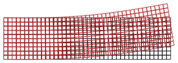
Sometimes one would like to model geometries that are under an initial stress (e.g. a pre-stressed beam that will be un-stressed once a load is applied). To pre-stress one can use:

preStress = {Inactive[
      Div][({{0, -((Y \[Nu])/(1 - \[Nu]^2))}, {-((Y (1 - \[Nu]))/(2 \
(1 - \[Nu]^2))), 0}}.Inactive[Grad][v[x, y], {x, y}]), {x, y}] + 
    Inactive[Div][
     Inactive[
       Plus][({{-(Y/(1 - \[Nu]^2)), 
          0}, {0, -((Y (1 - \[Nu]))/(2 (1 - \[Nu]^2)))}}.Inactive[
          Grad][u[x, y], {x, y}]), {{0}, {0}}], {x, y}], 
   Inactive[
      Div][({{0, -((Y (1 - \[Nu]))/(2 (1 - \[Nu]^2)))}, {-((Y \
\[Nu])/(1 - \[Nu]^2)), 0}}.Inactive[Grad][u[x, y], {x, y}]), {x, y}] +
     Inactive[Div][
     Inactive[
       Plus][({{-((Y (1 - \[Nu]))/(2 (1 - \[Nu]^2))), 
          0}, {0, -(Y/(1 - \[Nu]^2))}}.Inactive[Grad][
         v[x, y], {x, y}]), {{ss}, {0}}], {x, y}]};

Note that now we have added a `+ {{ss},{0}} to the second equation (for completeness I added a {{0},{0}} to the first one as well)

Inspecting what is parsed one gets:

{state} = 
  NDSolve`ProcessEquations[{preStress == {0, 0}, 
     DirichletCondition[u[x, y] == 0, x == 0], 
     DirichletCondition[v[x, y] == 0, x == 0]} /. 
    materialParameters, {u, v}, {x, y} \[Element] mesh];
state["FiniteElementData"][
  "PDECoefficientData"]["LoadDerivativeCoefficients"]
{{{{0}, {0}}}, {{{5}, {0}}}}

And solving the equation:

{uif, vif} = 
  NDSolveValue[{preStress == {0, 0}, 
     DirichletCondition[u[x, y] == 0, x == 0], 
     DirichletCondition[v[x, y] == 0, x == 0]} /. 
    materialParameters, {u, v}, {x, y} \[Element] mesh];
dmesh = ElementMeshDeformation[mesh, {uif, vif}, "ScalingFactor" -> 1];
Show[{mesh["Wireframe"], 
  dmesh["Wireframe"[
    "ElementMeshDirective" -> Directive[EdgeForm[Red], FaceForm[]]]]}]

Which is the same as your example. Note that no boundary conditions on the right hand side were specified. This beam is pre-stressed.

I do not know how (if at all) one can achieve this with adding the stress equations as you did. I am not saying it's not possible but I don't know how.

A parser:

You could use something like this:

ClearAll[PlaneStress];
PlaneStress[{Y_, nu_}, {u_, v_}, X : {x_, y_}] := 
 Module[{pStress}, 
  pStress = -Y/(1 - 
       nu^2)*{{{{1, 0}, {0, (1 - nu)/2}}, {{0, nu}, {(1 - nu)/2, 
        0}}}, {{{0, (1 - nu)/2}, {nu, 0}}, {{(1 - nu)/2, 0}, {0, 1}}}};
  
  {Inactive[Div][pStress[[1, 1]].Inactive[Grad][u, X], X] + 
    Inactive[Div][pStress[[1, 2]].Inactive[Grad][v, X], X], 
   Inactive[Div][pStress[[2, 1]].Inactive[Grad][u, X], X] + 
    Inactive[Div][pStress[[2, 2]].Inactive[Grad][v, X], X]}
  ]
PlaneStress[{Y, nu}, {u[x, y], v[x, y]}, {x, y}]

{Inactive[Div][{{0, -((nu*Y)/(1 - nu^2))}, {-((1 - nu)*Y)/(2*(1 - nu^2)), 0}} . 
    Inactive[Grad][v[x, y], {x, y}], {x, y}] + 
  Inactive[Div][{{-(Y/(1 - nu^2)), 0}, {0, -((1 - nu)*Y)/(2*(1 - nu^2))}} . 
    Inactive[Grad][u[x, y], {x, y}], {x, y}], 
 Inactive[Div][{{0, -((1 - nu)*Y)/(2*(1 - nu^2))}, {-((nu*Y)/(1 - nu^2)), 0}} . 
    Inactive[Grad][u[x, y], {x, y}], {x, y}] + 
  Inactive[Div][{{-((1 - nu)*Y)/(2*(1 - nu^2)), 0}, {0, -(Y/(1 - nu^2))}} . 
    Inactive[Grad][v[x, y], {x, y}], {x, y}]}

Hope this helps.