MMA 12: Transient plane stress problem

Question

Based on the numerical example enter link description here which is proposed by @Hugh and @user21, then, I continue to solve transient plane stress problems (u[t, x, y]), howerver, time-dependent loading (i.e. DirichletCondition[v[t, x, y] == ss*t, x == L])does not work in MMA 12.

Description of the numerical problem:

Left side of the plate is fixed;

Right side of the plate is controlled by the time-dependent displacement in y direction, namely Dirichlet BCs.

Code

Needs["NDSolve`FEM`"];
L = 1;
h = 0.125;
(*Shear stress on beam*)
ss = 5;
reg = Rectangle[{0, -h}, {L, h}];
mesh = ToElementMesh[reg];
mesh["Wireframe"]
materialParameters = {Y -> 10^3, \[Nu] -> 33/100};


ps = {Inactive[
      Div][({{-(Y/(1 - \[Nu]^2)), 
         0}, {0, -((Y (1 - \[Nu]))/(2 (1 - \[Nu]^2)))}}.Inactive[
         Grad][u[t, x, y], {x, y}]), {x, y}] + 
    Inactive[
      Div][({{0, -((Y \[Nu])/(1 - \[Nu]^2))}, {-((Y (1 - \[Nu]))/(2 \
(1 - \[Nu]^2))), 0}}.Inactive[Grad][v[t, x, y], {x, y}]), { x, 
      y}], Inactive[
      Div][({{0, -((Y (1 - \[Nu]))/(2 (1 - \[Nu]^2)))}, {-((Y \
\[Nu])/(1 - \[Nu]^2)), 0}}.Inactive[Grad][u[t, x, y], {x, y}]), {
       x, y}] + 
    Inactive[
      Div][({{-((Y (1 - \[Nu]))/(2 (1 - \[Nu]^2))), 
         0}, {0, -(Y/(1 - \[Nu]^2))}}.Inactive[Grad][
        v[t, x, y], {x, y}]), {x, y}]};
 {uu, vv} = 
  NDSolveValue[{ps == {0, 0}, 
     DirichletCondition[v[t, x, y] == ss*t, x == L], 
     DirichletCondition[u[t, x, y] == 0, x == 0], 
     DirichletCondition[v[t, x, y] == 0, x == 0]} /. 
    materialParameters, {u, v}, {t, 0, 1}, {x, y} \[Element] mesh];

Answer 1

You'd need to make the PDE time dependent and give initial conditions:

{uu, vv} = 
  NDSolveValue[{{D[u[t, x, y], t], D[v[t, x, y], t]} + ps == {0, 0}, 
     u[0, x, y] == 0, v[0, x, y] == 0, 
     DirichletCondition[v[t, x, y] == ss*t, x == L], 
     DirichletCondition[u[t, x, y] == 0, x == 0], 
     DirichletCondition[v[t, x, y] == 0, x == 0]} /. 
    materialParameters, {u, v}, {t, 0, 1}, {x, y} \[Element] mesh];

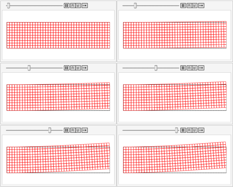
Here is a way to visualize that:

graphics = Function[t,
    dmesh = 
     ElementMeshDeformation[mesh, 
      Transpose[{uu[t, ##], vv[t, ##]} & @@@ mesh["Coordinates"]], 
      "ScalingFactor" -> 0.01];
    Show[{
      mesh["Wireframe"["MeshElement" -> "BoundaryElements"]],
      dmesh[
       "Wireframe"[
        "ElementMeshDirective" -> 
         Directive[EdgeForm[Red], FaceForm[]]]]
      }, PlotRange -> {{0, 1.}, {0.2, -0.2}}]] /@ Range[0, 1, 0.1];
ListAnimate[graphics]

You need to make sure that the material parameters match (I have used a ScaleFactor < 1 to make this specific example work. Use a smaller force or a stronger material)

If you want second order time derivatives, you'd also need to specify derivatives of the initial condition:

Monitor[{uu, vv} = 
  NDSolveValue[{{D[u[t, x, y], {t, 2}], D[v[t, x, y], {t, 2}]} + 
       ps == {0, 0}, u[0, x, y] == 0, v[0, x, y] == 0, 
     Derivative[1, 0, 0][u][0, x, y] == 0, 
     Derivative[1, 0, 0][v][0, x, y] == 0, 
     DirichletCondition[v[t, x, y] == ss*t, x == L], 
     DirichletCondition[u[t, x, y] == 0, x == 0], 
     DirichletCondition[v[t, x, y] == 0, x == 0]} /. 
    materialParameters, {u, v}, {t, 0, 10^-1}, {x, y} \[Element] mesh,
    EvaluationMonitor :> (monitor = 
      Row[{"t = ", CForm[t]}])], monitor]

Also, see the section A Swinging and Dynamically Loaded Beam that talks about Rayleigh damping.