Let's say I have a a very large list of data in the format {{n,f[n]}} so something like {{1,600},{2,700},{3,1100}...} and if this data is plotted, then it will look like a sum of Gaussian functions+a quadratic function when fitted (ie it will have multiple peaks, but it will be sitting on a quadratic curve). My goal is to remove the background, in this case probably a quadratic function so that the peaks sit on the horizontal axis. I have thought of a way to do this, but I cannot do the list manipulations. The method is basically look for the minimum data-value f[n] every 20 datapoints across (or bin of width 20). Now in every bin we have one 'minimum' datapoint. Then for every bin, search for all datavalues that is at least 6sigma higher than its corresponding 'minimum' datapoint(sigma is Sqrt[f[n]], and add these 'high' points to a list called background. If a 'high' point doesn't exist within the bin, add the minimum datapoint to background instead. Now we have a list of background points which are essentially points which 'hug' the bottom of the dataset, and the low outliers are removed
3 Answers
So imagine you do not know the background formula. This can be done in a beautiful way with FindFormula. Generate data:
f[x_] := Exp[-(x - 7)^2] + Exp[-(x + 5)^2] - .002 x^2
data = Table[{x, f[x] + .1 RandomReal[{-1, 1}]}, {x, -15, 15, .1}];

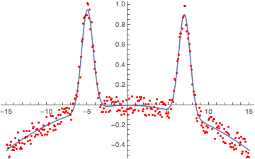
Plot[f[x], {x, -15, 15},
PlotRange -> All, Epilog -> {Red, Point[data]}]
Now use FindFormula to learn function form data and compare:
g = FindFormula[data, x,
SpecificityGoal -> 8,
TargetFunctions -> {Exp, Power, Plus, Times}]
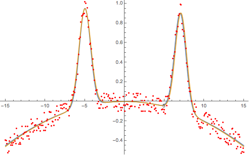
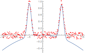
While I did make assumptions about potential functions, the exact combination is unknown and assumptions allow a lot of freedom for various models to be be tested.
Plot[{f[x], g}, {x, -15, 15},
PlotRange -> All, Epilog -> {Red, Point[data]}]
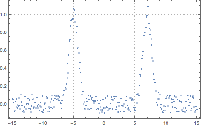
Now subtract background:
bg[x_] = g[[3]]
-0.002047501287539021` x^2

ListPlot[data /. {x_Real, y_Real} -> {x, y - bg[x]},
 PlotRange -> All, PlotTheme -> "Detailed"]
A common approach is to blank/mask out the signal and fit a polynomial to the remaining data. A problem to avoid here is overfitting, i.e. fitting some high-order polynomial to the noise structure.
Taking the artifical data from Vitaliy's answer:
f[x_] := Exp[-(x - 7)^2] + Exp[-(x + 5)^2] - .002 x^2
data = Table[{x, f[x] + .1 RandomReal[{-1, 1}]}, {x, -15, 15, .1}];
I select a mask for the signal from the plot:
windows = {{-7, -3}, {5, 9}};
blankedData = Select[data, Not@Between[#[[1]], windows] &];
And then fit a 2nd order polynomial:
baseline = Function[x, Evaluate@Fit[blankedData, {1, x, x^2}, x]]
function[x, 0.000152355 + 0.000454758 x - 0.00194731 x^2]
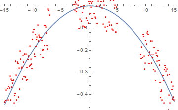
The background data:
Plot[baseline[x], {x, -15, 15}, PlotRange -> All, Epilog -> {Red, Point[blankedData]}]
noBaselineData = {#[[1]], #[[2]] - baseline[#[[2]]]} & /@ data;
Plot[f[x], {x, -15, 15}, PlotRange -> All,  Epilog -> {Red, Point[noBaselineData]}]
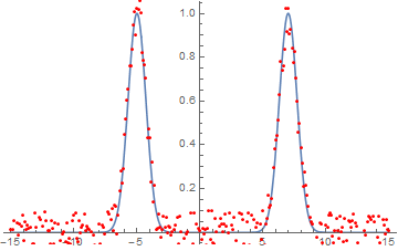
Now we fit the two peaks, with some reasonable starting values:
model = Exp[-(x - a)^2] + Exp[-(x + b)^2];
fit = FindFit[noBaselineData, model, {{a, 6}, {b, -10}}, x, Method -> NMinimize]
{a -> 6.99327, b -> 5.01227}
Plot[model /. fit, {x, -15, 15}, PlotRange -> All, Epilog -> {Red, Point[noBaselineData]}]
-
$\begingroup$ Small typo in the code:
...noBaselineData = ... - baseline[#[[2]]]}...should be... baseline[#[[1]]]}...$\endgroup$– BulatCommented Jun 1, 2018 at 19:10
If you know the number of Gaussians, you can proceed as follows.
Here is data with a single Gaussian added to a quadratic with noise:
mydata = Table[
  {n, .01 n^2 + 40 PDF[NormalDistribution[10, 1], n] + 3 RandomReal[]},
    {n, 1, 40}];
Here's a non-linear model of the assumed form but unknown constants:
nlm = NonlinearModelFit[
   mydata, {a n^2 + b PDF[NormalDistribution[c, d], n]},
   {a, b, c, d}, n]
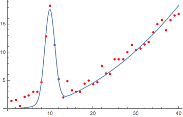
Here is a plot of the data and the non-linear fit:
Show[
    ListPlot[mydata, PlotStyle -> Red],
    Plot[nlm[n], {n, 0, 40}]
    ]
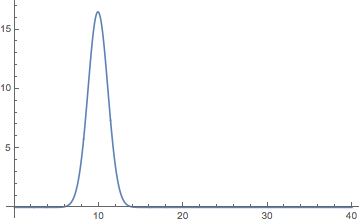
Now we subtract the "background" (quadratic term from the non-linear fit):
Plot[nlm[n] - .0114867 n^2, {n, 0, 40}, PlotRange -> All]
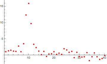
Here's the original data with the "background" subtracted:
myfixeddata =
 Table[{n, .01 n^2 + 40 PDF[NormalDistribution[10, 1], n] +
   3 RandomReal[] - .0114867 n^2},
   {n, 1, 40}];

ListPlot[myfixeddata, PlotRange -> All, PlotStyle -> Red]
-
$\begingroup$ I do not know the number of Gaussians $\endgroup$ Commented Oct 30, 2015 at 3:50


EstimatedBackground$\endgroup$