I have found the Bounded option useful in the SmoothKernelDistribution function, but I can't find any documentation for exactly how it is generating the bounded version of the distribution. Is there someplace I can go to find this? Thank you.
1 Answer
This deserves a little explanation since I found that the behavior is sometimes inconsistent.
Take some very simple data and create a function bound that illustrates how we suspect the bounded method is working (by reflecting the data about the bound, computing the estimate with the given bandwidth, and then truncating at the bound).
data = {1, 2, 3};

bound[data_, bw_] :=
     TruncatedDistribution[{0, Infinity},
          SmoothKernelDistribution[Join[-data, data], bw]]
Comparing to the built-in seems to indicate we are on the right track.
NIntegrate[(PDF[bound[data, 1/2], x] -
    PDF[SmoothKernelDistribution[data, 1/2, {"Bounded", 0, "Gaussian"}], x]
       )^2, {x, 0, Infinity}]

(* 1.27734*10^-9 *)
In my testing, this generally seems to hold unless the bandwidth is left as Automatic. In that case, it appears the bandwidth is half that for unbounded estimates (which I consider a bug).
bws = {"Scott", "Silverman", 3, Automatic};

(SmoothKernelDistribution[data, #]["Bandwidth"]/
    SmoothKernelDistribution[data, #, {"Bounded", 0, "Gaussian"}][
     "Bandwidth"]) & /@ bws

(* {1., 1., 1., 2.} *)
My recommendation would be to select a bandwidth by running the estimator unbounded and then feeding that back in as a bandwidth for the bounded estimator. For example...
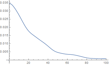
data = RandomVariate[ExponentialDistribution[1/25], 1000];
bw = SmoothKernelDistribution[data]["Bandwidth"];
est = SmoothKernelDistribution[data, bw, {"Bounded", 0, "Gaussian"}];

Plot[PDF[est, x], {x, -1, 100}]
-
$\begingroup$ Hi Andy, Thank you so much for taking time with this. After experimenting more with your code and mine, it seems to me that there is a bug in the way "Bounded" is implemented, at least in the case with a fixed lower bound and an upper bound of Infinity. The bug seems to result in a density that integrates to 1/2 instead of 1. The fix is easy -- just multiply by 2. Using "Bounded" with a lower bound of -Infinity and a fixed upper bound seems to work fine. $\endgroup$ Commented Jul 26, 2015 at 21:12
-
$\begingroup$ It makes some sense to me that this bug could happen because after doubling the data and then truncating, one would need to multiply the resulting density by 2. It seems that the code does not take this final step when there is a lower bound but no upper bound specified. $\endgroup$ Commented Jul 26, 2015 at 21:12


SmoothKernelDistribution? $\endgroup$