How to list plot data where the slope determines if it is plotted from a list of data?

Question

I am trying to listplot data from a list of data where the slope of the curve determines if it is plotted.

Example: Lets say the data measured is of the form x^2. I measure this data multiple times and gather multiple curves like this: Plot[{x^2, 10 x^2, 2 x^2, 12 x^2}, {x, 0, 10}]

Clearly there are two groups of slopes or curves. However, I would like to be able to list plot only the ones that cluster together based on the slope. Therefore, I would only want to plot {1x^2,2x^2} and {10x^2,12x^2}.

My thoughts are to use Find fit then Find cluster. However I am not sure how to Plot the curve that generated the slopes in each cluster.

Answer 1

First we have to generate some sample data to work with:

Clear[a, x];
polynomials = RandomInteger[100, 20] x^2;
noisyData[poly_] := poly /. x -> Range[0.1, 10, 0.1] + RandomReal[0.1, 100]
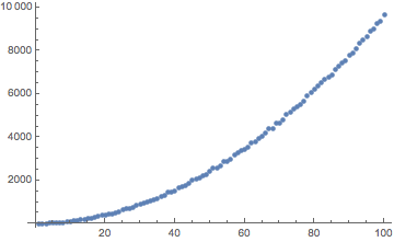
ListPlot@noisyData[First@polynomials]

This represents the noisy data that you have obtained somehow. Note that I'm supposing a sample frequency of 10 samples per unit step. So on the x axis it says 100, but actually if the x axis represented time it would only say 10. In order to fit this data we have to supply the x coordinate corresponding every measurement.

data = Transpose[{Range[0.1, 10, 0.1], noisyData[First@polynomials]}];
r = FindFit[data, a x^2, a, x]
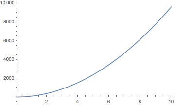
Plot[a x^2 /. r, {x, 0, 10}]
(* Out: {a -> 96.2328} *)

The actual coefficient in the example above is 95, but it was estimated to 96.2. Let's find the estimate of all polynomials:

data = Transpose[{Range[0.1, 10, 0.1], noisyData[#]}] & /@ polynomials;
estimates = FindFit[#, a x^2, a, x] & /@ data;
clusters = FindClusters[a /. estimates]
(* Out: {{96.2559, 94.0996, 85.1444, 100.196}, {74.8276, 63.7454, 70.7918, 
  77.9841, 72.85, 77.9613}, {41.5601, 48.6428, 57.6537, 47.627, 
  51.5892, 56.6536}, {21.2733, 29.4381, 22.2827, 12.1583}} *)

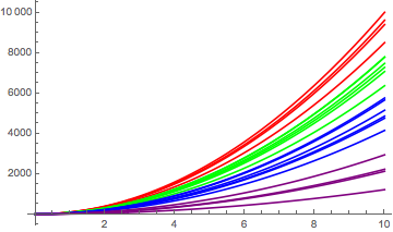
Here I've used FindClusters to let Mathematica sort the polynomials into suitable groups. As you can see in the result it found four groups of polynomials. We can plot them to verify our results:

fittedPolynomials = clusters x^2;
Show@MapThread[
  Plot[#, {x, 0, 10}, PlotStyle -> #2] &,
  {fittedPolynomials, {Red, Green, Blue, Purple}}
  ]

In this example I have specified four colors because I have four groups of polynomials. You will have to supply as many colors as you need.