Numerical Integration different in Mathematica version 9 and 10 with same options

Question

I have noted that the same function with the same settings gives me different results in Mathematica version 9 and 10. This involves integrating numerically interpolating functions and so on. Here a minimal working example:

kmin=3/400;
kmax=5;

wk[x_] := 3*x^-3*(Sin[x] - x*Cos[x]);

myIntegrationFunction[ps_, scal_?NumericQ] := NIntegrate[
 Exp[3 lk]*ps[Exp@lk]*wk[Exp[lk]*scal]^2, {lk, Log[kmin], 
 Log[10*kmax]}, MaxRecursion -> 15, PrecisionGoal -> 4, 
 AccuracyGoal -> 4];

interptab = Table[{x, -x^2 + 3 x - 1}, {x, 0.001, 10, 0.01}];

interpFunc = Interpolation[interptab]

myIntegrationFunction[interpFunc, 8]

In Mathematica 10.0.2.0 I get:

>>> -0.0439862

In Mathematica 9.0.1.0 I get:

>>> -0.0435323

The error is more than 1%.

I know that the PrecisionGoal is 4 and Accuracy Goal is also 4 and the error is in the 5th digit. But if in Mathematica 10 I run this integral using AccuracyGoal->6, I get the same result as in Mathematica 9 using AccuracyGoal->4, namely: -0.0435323.

So I wanted to ask to the experts here, what has changed in the options between v9 and v10?

In my real life case, I have to interpolate complicated data and I don't want to have to increase AccuracyGoal in v10 if I can get a good and faster result in v9.

Thanks!

Answer 1

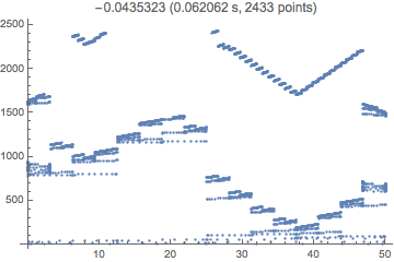
In V10 there has been added some symbolic processing of integrands containing an InterpolatingFunction. In particular if the interpolation grid divides the domain of integration into a number of subintervals, the number being at most the value of the option "MaxSubregions", the integrand will automatically be integrated over each subinterval. In V9, this is done only if Method -> "InterpolationPointsSubdivision" is used. The number of grid points in interpFunc is quite large,

Length[interpFunc["Grid"]]
(*  1000  *)

so the impact on timing is also quite large.

We can see what happens with the following function adapted from the NIntegrate tutorials and a slight redefinition of myIntegrationFunction to Sow the sample abscissae and accept NIntegrate options.

SetAttributes[samplePlot, HoldAll];
samplePlot[integral_] := Module[{sampledPoints, time, value},
   sampledPoints = Reap[ {time, value} = AbsoluteTiming[integral] ][[2, 1]];
   ListPlot[Transpose[{sampledPoints, Range[Length[sampledPoints]]}], 
    PlotLabel -> Row[{value, " (", time, " s, ", Length[sampledPoints], " points)"}]]
   ]; 

Clear[myIntegrationFunction];
myIntegrationFunction[ps_, scal_?NumericQ, opts : OptionsPattern[NIntegrate]] := 
  NIntegrate[
   Exp[3 lk]*ps[Exp@lk]*wk[Exp[lk]*scal]^2,
   {lk, Log[kmin], Log[10*kmax]},
   opts, (* MaxRecursion -> 15, (* unneeded for this example *) *)
   PrecisionGoal -> 4, AccuracyGoal -> 4, EvaluationMonitor :> Sow[lk]];

OP's computations

V9:

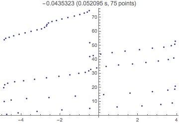
samplePlot[myIntegrationFunction[interpFunc,8]]

V10:

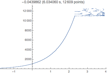
samplePlot[myIntegrationFunction[interpFunc, 8]]

The recursive subdivision for lk > Log[10] happens because Exp[lk] goes beyond the domain of the interpolation. Thus extrapolation is being used; and instead of the normal InterpolatingFunction strategy we see on the left, NIntegrate is computing a normal numerical integral. The reason the plot looks smooth on the left side is that the Gauss-Kronrod method is applied once on each of the 1000 subintervals (at 11 sample points each). The estimated error of each of the sub-integrals is so small that the "GlobalAdaptive" strategy never goes back to subdivide them further.

Mimicking V9 behavior (V10 solution)

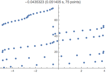
One can create a black-box wrapper for the interpolating function. Then NIntegrate won't see the InterpolatingFunction and it will choose a different strategy, apparently the same one as V9. It will be seen that this is preferable to "SymbolicProcessing" -> None.

myif[u_?NumericQ] := interpFunc[u];
samplePlot[myIntegrationFunction[myif, 8]]

Compare with "SymbolicProcessing" -> None:

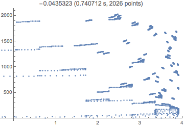
samplePlot[myIntegrationFunction[interpFunc, 8,
  Method -> {"GlobalAdaptive", "SymbolicProcessing" -> None}]]

NIntegrate::slwcon: Numerical integration converging too slowly; suspect one of the following: singularity, value of the integration is 0, highly oscillatory integrand, or WorkingPrecision too small. >>

One can simplify this integral with a substitution u = Exp[lk], which might be the reason that symbolic processing helps this particular example. It's not clear that one can generalize.

Using "MaxSubregions" is not optimal

Setting "MaxSubregions" to any positive integer less than Length[interpFunc["Grid"]] prevents subdivision at the grid points. The value computed in this case is accurate, but the speed is somewhat slow.

samplePlot[
 myIntegrationFunction[interpFunc, 8,
  Method -> {"InterpolationPointsSubdivision", "MaxSubregions" -> 1}]
 ]

NIntegrate::slwcon: Numerical integration converging too slowly; suspect one of the following: singularity, value of the integration is 0, highly oscillatory integrand, or WorkingPrecision too small. >>

Performing the substitution helps, suggesting that NIntegrate might handle interpolating functions in the simple form if[u] better than in composition such as if[Exp[lk]] (but see concluding remarks below).

samplePlot[
 Block[{ps = interpFunc, scal = 8, nreg = 1},
  NIntegrate[u^2*ps[u]*wk[u*scal]^2, {u, kmin, 10*kmax},
   PrecisionGoal -> 4, AccuracyGoal -> 4,
   Method -> {"InterpolationPointsSubdivision", "MaxSubregions" -> nreg},
   EvaluationMonitor :> Sow[u]]]
 ]

It is interesting that it is much faster even though the total number of functions evaluations is greater.

Concluding remarks

If one is interpolating noisy data, the default V10 method is likely to produce more accurate results (that is, integrate the interpolation accurately) and less likely to complain about convergence. Given that the range of use-cases here could be quite wide, it is important to realize that the appropriate integration strategy depends on the integrand. The solution above works in this special case, and it should in general give the V9 behavior. But mimicking V9 is probably not always the best solution. (Note in particular that the OP's interpolation is a cubic interpolation of a cubic polynomial. The interpolation agrees exactly with the polynomial, even under extrapolation, and is a smooth function with well-behaved derivatives. It should be expected that the OP's integral would be easy to compute numerically, even more so after the substution u = Exp[lk].)