MinRecursion changes result of integration by 100 orders of magnitude

Question

I want to compute a triple integral. I did it using two codes: the first is NIntegrate[2 1/2 ((50^2 - (((u - v)/2)^2 + t^2 + m^2) Log[ (50^2 + (u - v)^2/4 + t^2 + m^2)/((u - v)^2/4 + t^2 + m^2)])/Log [ ((u + v)^2/4 + t^2 + m^2 + 50^2)/(((u + v)/2)^2 + t^2 + m^2)] ) Exp[-(u)^2/(2 10^-3)], {v, 0, 50 Sqrt[2]},{u, v - 2 50 , -v + 2 50 }, {t, -50, 50}, WorkingPrecision -> 15, MinRecursion -> 8, PrecisionGoal -> 5, AccuracyGoal -> 5]

Where m is a constant equal to 0.1. Notice that the integrand is bounded and smooth in the domain of integration. The only thing is that it has a smooth peak at the u=0 plane.

This gives me no error message, and the result 5675.53769275483. Now i try with the same code, but without specifying MinRecursion, and the result is(again with no error messages) 2.44759996103605*10^(-132) !

How can I rely in such a result?? Anyone knows what is going on?

Also, setting MinRecursion to 4 and varying PrecisionGoal and AccuracyGoal i get different results. E.g. for Precision and Accuracy equal to 8 I get 75853.6468454678, and for Precision=Accu=10 I get 134823.121278000.

Answer 1

Why is this a hard integral

Numerical computations have to work with finite sampling, finite steps, and so forth. So it's possible that a given sampling will miss important features as well as fool error estimates.

Let

integrand = (* OP's integrand *)

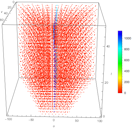
We'll analyze just one of the OP's results to give an idea of where the important features are. We'll take all the sample abscissae used by NIntegrate and color the points by the value of the integrand. (Luckily, it's only a 3D integral; if higher, this would be hard to visualize.)

Block[{m},
 m = 1/10;
 {res, {abs}} = 
  Reap@NIntegrate[                          (* Reap collects sample abscissae *)
    integrand,
    {v, 0, 50 Sqrt[2]}, {u, v - 2 50, -v + 2 50}, {t, -50, 50},
    MinRecursion -> 4,
    EvaluationMonitor :> Sow[{v, u, t}]];  (* Sow sows the sample abscissae *)
 res
 ]
(*  14811.2  *)

vals = Block[{m = 0.1},    (* get the function values *)
   integrand /. Thread[{v, u, t} -> Transpose@abs]];

Legended[    
 Graphics3D[    (* plot the abscissae colored by vals *)
  {PointSize[Small], 
   Point[abs, 
    VertexColors -> Hue /@ (0.7 Rescale[RealExponent@vals])]},
  BoxRatios -> {1, 1, 1}, Axes -> True, AxesLabel -> {v, u, t}, 
  ViewPoint -> {4, 0.15, 1.5}],
 BarLegend[{Hue[Rescale[#, MinMax@vals, {0., 0.7}]] &, MinMax@vals}]
 ]

The graphics show that most of the values of the integrand are near zero, except for a very narrow strip near u == 0. One needs sufficient subdivision near u == 0 to get enough sampling for the integral to be accurately estimated. That starts to happen around MinRecursion -> 4, but the level 4 is apparently not high enough. Plus it's inefficient.

How to do this integral

A better way is to look at the integrand and realize that the m^2 term in the denominator controls the width of the layer near u == 0 where the integrand is large. Then we can manually subdivide the region of integration just along the u axis thus:

Block[{m},
 m = 1/10;
 {res, {abs}} = Reap@NIntegrate[integrand,
    {v, 0, 50 Sqrt[2]},
    {u, v - 2 50, -10, -1, -m, 0, m, 1, 10, -v + 2 50}, (* extra subdivision *)
    {t, -50, 50},
    EvaluationMonitor :> Sow[{v, u, t}]];
 res
 ]
(*  544909.  *)

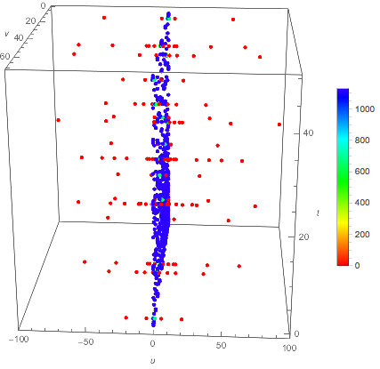
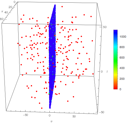
We can see that there is far few samples away from plane u == 0 and much denser sampling it.

Check

One can check with the Monte Carlo method:

Block[{m},
 m = 1/10;
 {res, {abs}} = Reap@NIntegrate[integrand,
    {v, 0, 50 Sqrt[2]}, {u, v - 2 50, -1, -m, 0, m, 
     1, -v + 2 50}, {t, -50, 50},
    Method -> {"MonteCarlo", "RandomSeed" -> 0},
    EvaluationMonitor :> Sow[{v, u, t}]];
 res
 ]
(*  550004.  *)

You can vary the random seed to see that the value bounces above and below 544,000.

Why the OP's basic NIntegrate fails

The multidimensional rule of NIntegrate in fact initially samples along the plane u == 0, so why does it report an integral on the order of 10^-132? To explain this, we'll use IntegrationMonitor and EvaluationMonitor. The IntegrationMonitor gets called every time there is a recursive subdivision of an integration subregion. We can use it to signal the EvaluationMonitor what level of recursive subdivision we're at. This works for this example because the integration does only one subdivision.

First note that NIntegrate maps the integration region to a unit cube. In the "MultidimensionalRule", the basic sampling in a three-dimensional integral using 5 generators (the default) consists of 33 points symmetrically placed about the unit cube. It is an open sampling, that is, none of the points lie on the surface of the cube. When a subregion is divided, the old sampling points and function values are discarded, the region is split in half along one of the axes determined by the algorithm, and each half is sampled again with the sampling of the unit cube being scaled to the cuboid subregion.

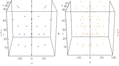
In the initial sampling, one can see below that large values near u == 0 are found. The algorithm then determines to subdivide along the u axis. The second sampling results in extremely small function values that translate to an extremely small value for the integral and for its error estimate. The small values occur because the region is divided along the plane u == 0 and the open sampling is too far from the plane to yield large integrand values.

Block[{m},
 m = 1/10;
 level = 1;
 {res, abslev} = Reap[
   NIntegrate[integrand,
    {v, 0, 50 Sqrt[2]}, {u, v - 2 50, -v + 2 50}, {t, -50, 50},
    WorkingPrecision -> 15, (*MinRecursion->8,*)
    PrecisionGoal -> 5, AccuracyGoal -> 5,
    IntegrationMonitor :> (++level &),            (* increment level *)
    EvaluationMonitor :> Sow[{v, u, t}, level]],  (* Sow[] points acc. to level *)
   Range@9]; (* Need only levels  {1, 2};  Ragne[9] was for safety *)
 res
 ]
(*  2.37965207993096*10^-132  *)

(* Show samplings *)
MapIndexed[   (* map each level of sampling points *)
 Graphics3D[{
    {Opacity[0.2], Black, InfinitePlane[{0, 0, 0}, {{1, 0, 0}, {0, 0, 1}}]},
    PointSize[Medium], {ColorData[97][First@#2], 
     PointSize[0.06/(2 + First@#2)], Point /@ #}
    },
   Axes -> True, AxesLabel -> {v, u, t}, BoxRatios -> {1, 1, 1}, 
   ViewPoint -> {4, 0.0, 1.5}
   ] &,
 abslev[[;; level - 1]]
 ]

The values away from u == 0 are amazingly small:

vals1 = integrand /. Thread[{v, u, t} -> Transpose@abslev[[1, 1]]] /. m -> 1/10;
vals2 = integrand /. Thread[{v, u, t} -> Transpose@abslev[[2, 1]]] /. m -> 1/10;

(* Median exponents base 10 *)
vals1 // RealExponent // Median
vals2 // RealExponent // Median
(*
-167144.
-226858.
*)

(* At machine precision, most values underflow to zero in V11.3 *)
vals1 // N
vals2 // N
(*
{986.64, 1020.42, 955.617, 1071.58, 928.533, 0., 0., 0., 0., 1046.01, 
 914.651, 1113.91, 826.08, 0., 0., 0., 0., 1139.7, 1018.93, 358.936,
 1101.42, 0., 0., 0., 0., 0., 0., 0., 0., 0., 0., 0., 0.}

{0., 0., 0., 0., 0., 0., 0., 0., 0., 0., 0., 0., 0., 5.22486*10^-136, 0.,
 0., 0., 0., 0., 0., 0., 0., 0., 0., 0., 0., 0., 0., 0., 0., 0., 0., 0.,
 0., 0., 0., 0., 0., 0., 0., 0., 0., 0., 0., 0., 0., 0., 5.42339*10^-136,
 0., 0., 0., 0., 0., 0., 0., 0., 0., 0., 0., 0., 0., 0., 0., 0., 0., 0.}
*)

Here are the integral and error estimates of each level:

Block[{m},
 m = 1/10;
 {res, {mon}} = Reap@NIntegrate[integrand,
    {v, 0, 50 Sqrt[2]}, {u, v - 2 50, -v + 2 50}, {t, -50, 50},
    WorkingPrecision -> 15,(*MinRecursion->8,*)
    PrecisionGoal -> 5, AccuracyGoal -> 5,
    IntegrationMonitor -> (Sow[
        Total@Map[{#1@"Integral", #1@"Error"} &, #1]] &)];
 res
 ]
(*  2.37965207993096*10^-132  *)

mon
(* integral                   error
  {{1.76258423545017*10^8,    4.18095426422557*10^8},      initial
   {2.37965207993096*10^-132, 5.65167368983603*10^-132}}   after subdivision
*)

Note that the relative error of the final result is huge, but because the AccuracyGoal is set to 5, any error less than 10^-5 is acceptable. Hence NIntegrate terminates after just one subdivision.