Determining which rule NIntegrate selects automatically

Question

I need to numerically integrate a highly oscillatory function over the semi-infinite domain $(0,\infty)$:

$$\int_0^\infty \frac{\sin^2(x) \sin^2(1000 x)}{x^{5/2}}\mathrm dx$$

Since the Levin rule (which was recently added to Mathematica, starting in version 8) was developed specifically for oscillatory integrals such as this, I thought I'd try it:

ans = NIntegrate[Sin[x]^2 Sin[1000 x]^2/x^(5/2), {x, 0, Infinity}, 
                 Method -> {"LevinRule"}, PrecisionGoal -> 8, MaxRecursion -> 30]

Using an exact solution for this integral, I can confirm the relative accuracy of the Mathematica result is $1 \times 10^{-11}$, and moreover the calculation is very quick. At first, this led me to believe that Levin's method works great for this problem, but...

It turns out that Mathematica must be automatically switching to non-oscillatory rule behind the scenes, because forcing it not to do so gives a very poor result:

ans = NIntegrate[Sin[x]^2 Sin[1000 x]^2/x^(5/2), {x, 0, Infinity},  
                 Method -> {"LevinRule", "MethodSwitching" -> False},
                 PrecisionGoal -> 8, MaxRecursion -> 30]

NIntegrate::ncvb: NIntegrate failed to converge to prescribed accuracy after 30 recursive bisections in x near {x} = {0.}. NIntegrate obtained -3497.5 and 3510.0321785369356` for the integral and error estimates. >>

Is there any way to find out which alternative non-oscillatory rule Mathematica is automatically selecting? I've tried to guess which rule is being used by manually specifying few rules but the results I've obtained with other rules are inaccurate, slow, or both:

ans = NIntegrate[(Sin[x])^2 (Sin[1000 x])^2/x^(5/2), {x, 0, Infinity}, 
                 Method -> "ClenshawCurtisRule", AccuracyGoal -> 8, MaxRecursion -> 30]

NIntegrate::slwcon: Numerical integration converging too slowly; suspect one of the following: singularity, value of the integration is 0, highly oscillatory integrand, or WorkingPrecision too small. >>

NIntegrate::eincr: The global error of the strategy GlobalAdaptive has increased more than 400 times. The global error is expected to decrease monotonically after a number of integrand evaluations. Suspect one of the following: the working precision is insufficient for the specified precision goal; the integrand is highly oscillatory or it is not a (piecewise) smooth function; or the true value of the integral is 0. Increasing the value of the GlobalAdaptive option MaxErrorIncreases might lead to a convergent numerical integration. NIntegrate obtained 0.000013202052151832003` and 1.0480362255168103`*^-6 for the integral and error estimates. >>

I'd like to know what rule Mathematica is using so that I can try adjusting options for the best performance possible. I need to calculate this integral several hundred thousand times, as the innermost integral of a nested double integration. Furthermore, when it comes to publishing my results, I would like to be able to state the integration strategy that was actually used, rather than "Mathematica knew how to handle it".

Answer 1

This question comes up often enough. See this discussion at community.wolfram.com : Integration method used in NIntegrate , and the notebook Finding the applied NIntegrate methods attached to my second response in the discussion.

That notebook contains examples of usage of the undocumented function NIntegrateSamplingPoints and NIntegrate's option IntegrationMonitor.

The integral in the question

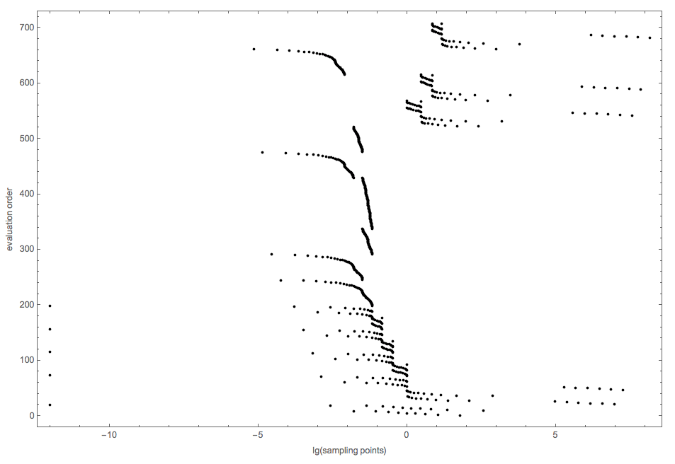
For the integral in the question with NIntegrateSamplingPoints we get kind of a boring picture because of the infinite region. Taking logs of the sampling points might be more informative:

Needs["Integration`NIntegrateUtilities`"]

gr = NIntegrateSamplingPoints@
   NIntegrate[Sin[x]^2 Sin[1000 x]^2/x^(5/2), {x, 0, Infinity}, 
    Method -> {"LevinRule", 
      Method -> {"GaussKronrodRule", "Points" -> 11}}];

Graphics[gr[[1]] /. 
  Point[{x_?NumericQ, y_?NumericQ}] :> 
   Point[{Log[10, x + 10^-12], y}], Frame -> True, 
 FrameLabel -> {"lg(sampling points)", "evaluation order"}, AspectRatio -> 1/1.5]

The plot shows the order of evaluation of the sampling points.

Using IntegrationMonitor we can see the application of the integrand over the regions derived with the LevinRule method:

t = Reap[NIntegrate[Sin[x]^2 Sin[1000 x]^2/x^(5/2), {x, 0, Infinity}, 
    Method -> {"LevinRule", 
      Method -> {"GaussKronrodRule", "Points" -> 11}}, 
    PrecisionGoal -> 1.5, 
    IntegrationMonitor -> (Sow[
        Map[{#1@"Integrand", #1@"Boundaries", #1@"Integral", #1@
            "Error"} &, #1]] &)]];
res = t[[1]];
t = t[[2, 1]];
t

UPDATE

(I have had the code below for some time, but I have been hesitant to share it because of several concerns. It is somewhat hard to interpret its results and coming up with it does require some internal knowledge of NIntegrate's development. After dedicated discussions with/about the NIntegrate method tracing code at WTC 2015 it seems that it is better to show and describe it.)

We can trace NIntegrate's method initialization by manipulating the top level initialization function implementations. The basic idea is to take the down values and up values of the initialization functions of NIntegrate's methods that have the form

Block[{v___}, b_CompoundExpression]

and replace them with

Block[{res = Block[{v}, b]}, Print[res]; res]

When an NIntegrate command is executed we will see a printed trace of the methods that are initialized.

Here is the tracing code:

symbNames = Names["NIntegrate`*"];
symbNames = 
  Append[Pick[symbNames, 
    StringMatchQ[
     symbNames, (__ ~~ "Rule") | (__ ~~ 
        "Global" | "Local" | "MonteCarlo" | "Principal" | "Levin" | 
         "Osc" ~~ ___)]], "NIntegrate`AutomaticStrategy"];
symbs = ToExpression[#] & /@ symbNames;
dvs = DownValues /@ symbs;
uvs = UpValues /@ symbs;
Unprotect /@ symbs;
dvsNew = MapThread[
   With[{s = #2},
     DownValues[s] = 
      ReplaceAll[#1, 
       HoldPattern[
         a_ :> b___] :> (a :> (Print["DownValue call for: ", 
            Style[s, Red]]; b))]] &, {dvs, symbs, symbNames}];
uvsNew = MapThread[
   With[{s = #2},
     UpValues[s] =
      ReplaceAll[#1,
       HoldPattern[Block[vars_, CompoundExpression[b___]]] :>
        Block[{res = Block[vars, CompoundExpression[b]]}, 
         Print["UpValue call for: ", Style[s, Blue], 
          Style[" ::\n", Blue], res]; res]
       ]
     ] &, {uvs, symbs, symbNames}];

In that code using Pick I have reduced the number of NIntegrate context symbols being traced. Of course, if it is desired, the down/up values of the full list of the NIntegrate context symbols can be manipulated for tracing.

Let us look at tracing examples.

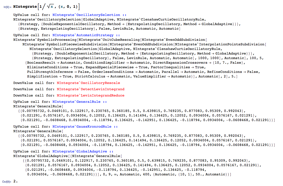
Here is a numerical integration computation with an automatically selected method:

The basic objects of NIntegrate are integration regions. Each region has its own integration function and integration rule. In order to interpret the printed trace it is helpful to know that NIntegrate uses the software design patterns Strategy, Composite, Decorator, and others.

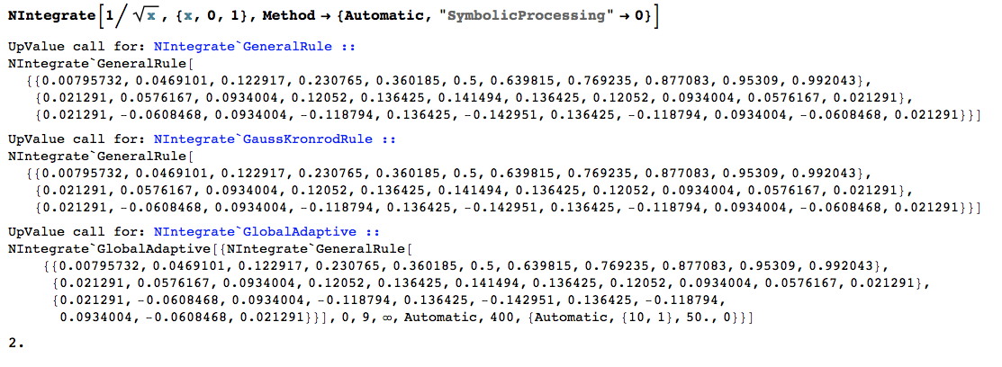
NIntegrate's symbolic pre-processors are using Decorator, and we can see in the trace that the outcome of AutomaticStrategy are pre-processor symbols wrapped around the method "GlobalAdaptive". The method "GlobalAdaptive" uses a Gauss-Kronrod rule, which after its initialization is treated as a general rule. (I.e. a list of abscissas, integral estimate weights, and approximation error weights.)

The method GlobalAdaptive is going to be directly used if symbolic processing is prevented:

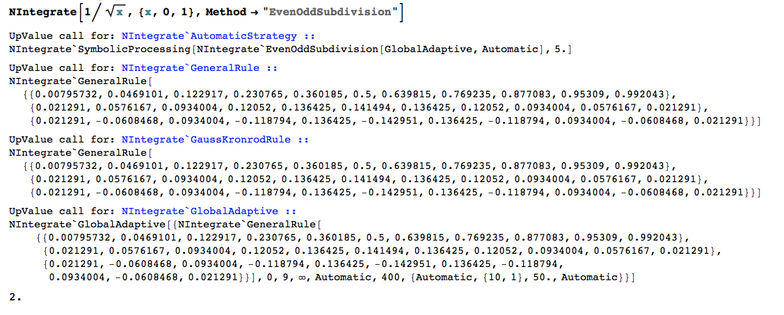
Here is a numerical integration computation with a specifically selected pre-processing method:

UPDATE 2 (IntegrationMonitor methods)

(Thanks to Michael E2 for prompting these explanations.)

Each integration strategy of NIntegrate creates and manipulates a collection of integration regions. Each integration region can have its own integrand and/or integration rule. NIntegrate's main integration strategy "GlobalAdaptive" keeps the integration regions in a heap according to their error. The sum of the integral estimates of all regions make the global integral estimate. The sum of the integral errors make the global error. If the global error is larger than the desired tollerance "GlobalAdaptive" splits the region with the largest error estimate into two regions and applies the integration rule. If too many splittings have been done then a singularity handler is applied over the last region split.

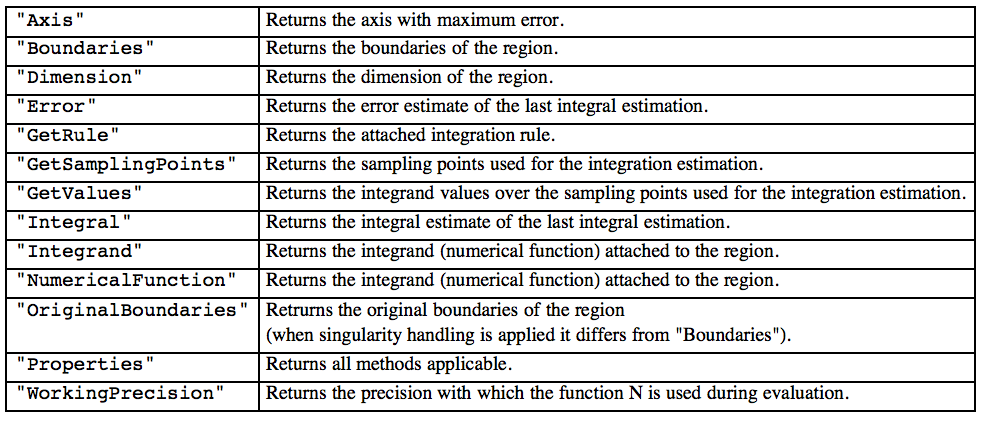
At each step of an integration strategy the option IntegrationMonitor obtains as an argument the list of integration regions used in that step. Below is a table that shows methods that can be applied to each integration region in that list.

And here is (another) example of the application of those methods:

iRegionMethods = {"Axis", "Boundaries", "Dimension", "Error", 
  "GetRule", "Integral", "Integrand", "WorkingPrecision"}; res = 
 Reap@NIntegrate[x^2 y^2, {x, 0, 4}, {y, 0, 2}, PrecisionGoal -> 1.1, 
   Method -> "AdaptiveMonteCarlo", 
   IntegrationMonitor :> 
    Function[{iregs}, 
     Sow[Association /@ 
       Transpose[
        Map[Thread[# -> Through[iregs[#]]] &, iRegionMethods]]]]];
Dataset[Flatten[res[[2]]]]

Answer 2

As you may know, the backup non-oscillatory rule is controlled by the Method sub-option of `"LevinRule", documented here. You can use it like this:

In[60]:= NIntegrate[Sin[x]^2 Sin[1000 x]^2/x^(5/2), {x, 0, Infinity}, 
 Method -> {"LevinRule", 
   Method -> {"GaussKronrodRule", "Points" -> 11}}]

Out[60]= 1.16762

With this, you can try to tune for performance.

In your example, the default setting Method -> Automatic is effectively equivalent to Method -> {"GaussKronrodRule", "Points" -> 5}. There is no documented method to determine this, but you can more or less verify it by doing something naughty like:

In[61]:= Block[{NIntegrate`GaussKronrodRuleData = (Print[{##}]; 
     Abort[]) &}, 
 NIntegrate[Sin[x]^2 Sin[1000 x]^2/x^(5/2), {x, 0, Infinity}, 
  Method -> {"LevinRule"}, PrecisionGoal -> 8, MaxRecursion -> 30]]

During evaluation of In[61]:= {5,MachinePrecision}

Out[61]= $Aborted