I will address the case of an irregular grid. There are two or three ways to produce a pretty good looking plot, through rescaling/FrameTicks or through interpolation. The ticks method involves rescaling the data. This is perhaps the easiest, but the resulting plot cannot be easily combined with other plots, since the underlying coordinates have been changed. The tick labels make appear, and only appear, that they haven't been changed. There are a couple of ways of constructing interpolations. Each is fairly easy but requires some work. We can restrict the domain to the outline of the grid or the convex hull of the grid.
The underlying issue
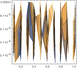
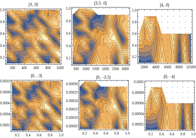
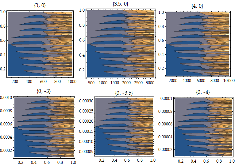
Both Interpolation[data] and ListContourPlot[data] construct an interpolation on the Delaunay triangulation of convex hull of the projection of data onto xy plane. Since the Delaunay triangulation maximizes the minimum interior angle, it is important to realize that the angle is measured as it usually is in Cartesian geometry. When we scale the image (which ListContourPlot does by setting the aspect ratio to 1), the angles are distorted. ListContourPlot probably tries to help, but like balancing too many plates, the plot comes crashing down:
Rescaling and/or resetting ticks
The undocumented function Charting`FindTicks is convenient (while it lasts -- but plotting functions will always need such a function). It styles the ticks in the default way. It also rescales the tick positions. The xy coordinates of the data are rescaled to span the interval {0, 1}. We get the ticks for the actual data range and rescale to {0, 1}.
trdata = Transpose[data];
ranges = Through[{Min, Max}[#]] & /@ Most@trdata;
plotdata = Transpose@MapAt[Rescale, trdata, {{1}, {2}}];
ListContourPlot[plotdata,
 FrameTicks -> ({#, None} & /@ (Charting`FindTicks[{0, 1}, {##}][0, 1] & @@@
      Reverse@ranges))]
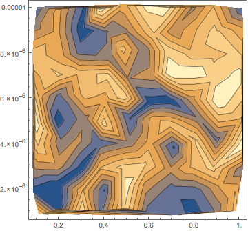
This may be more appealing: Scale data, plot, and rescale back:
Show[
 ListContourPlot[data.DiagonalMatrix[{1, 10^5, 1}]] /.
  GraphicsComplex[pts_, rest_] :>
   GraphicsComplex[pts.Inverse[DiagonalMatrix[{1, 10^5}]], rest],
 PlotRange -> All]
The plot looks like the one above.
Addendum: Manual ticks
myTicks[{primary_, secondary_}, range_] := Join[
  Map[{Rescale[#, range], N@#} &, primary],
  Map[{Rescale[#, range], "", {0.005`, 0.`}, {AbsoluteThickness[0.1`]}} &,
   Flatten[secondary, 1]]
  ]

ListContourPlot[plotdata,
 FrameTicks -> ({#, None} & /@ (myTicks[FindDivisions[#, {6, 6}], #] & /@
      Reverse@ranges))]
This manual approach is fairly straightforward. My main issue is formatting numbers, which I find a great waster of time.
Interpolations
For a slightly irregular grid we can construct an interpolation in a few ways. First, let's set up some random data whose bounding box has an extreme aspect ratio; from the data we'll extract the grid (domain) and values (range).
SeedRandom[1];
data = Flatten[
   Table[{10^-1, 10^-6, 1} *    (* scaling factors *)
       {i + RandomReal[{-0.2, 0.2}], j + RandomReal[{-0.2, 0.2}], RandomReal[{1, 5}]},
     {i, 10}, {j, 10}], 1];
grid = data[[All, {1, 2}]];
values = data[[All, 3]];
Why Interpolation does not work well
The straight use Interpolation is possible but has problems. The option "ExtrapolationHandler" can be used to restrict the domain to the convex hull:
ifInt = Interpolation[data, InterpolationOrder -> 1,
   "ExtrapolationHandler" -> {Indeterminate &, "WarningMessage" -> False}];
We can see that the mesh is used is the same as DelaunayMesh:
GraphicsRow[{
  Show[DelaunayMesh[grid], AspectRatio -> 1],
  Show[ifInt["ElementMesh"]["Wireframe"], AspectRatio -> 1]
  }]
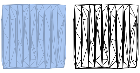
One can see that the distortion of the triangulation has consequences for the plot of ifInt.
ContourPlot[ifInt[x, y],
 Evaluate[Sequence @@ Transpose[Join[{{x, y}}, Transpose[ifInt["Domain"]]]]]]
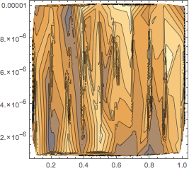
Tricking DelaunayTriangulation
We can use ToElementMesh to make an ElementMesh out of the Delaunay triangulation of the rescaled grid. From this we can make an interpolation with ElementMeshInterpolation, using the triangulation but substituting the unscaled grid for the coordinates.
meshdel = ToElementMesh[
   "Coordinates" -> grid,
   "MeshElements" -> {TriangleElement[
      MeshCells[DelaunayMesh[Transpose[Rescale /@ Transpose[grid]]], 2] /. Polygon[p_] :> p
      ]}
   ];

Show[meshdel["Wireframe"], AspectRatio -> 1, Frame -> True]
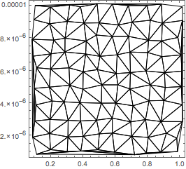
We can construct an interpolation like this:
ifdel = ElementMeshInterpolation[{meshdel}, values,
   "ExtrapolationHandler" -> {Indeterminate &, "WarningMessage" -> False}];

ContourPlot[ifdel[x, y],
 Evaluate[Sequence @@ Transpose[Join[{{x, y}}, Transpose[ifdel["Domain"]]]]]]
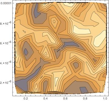
Probably the missing Method -> {"DelaunayDomainScaling" -> True} option did something similar.
Restricting to the grid outline
One issue with the Delaunay triangulation are some narrow triangles used to fill in the convex hull, which lead to some small ugly shadows along the edges of the plot. With a little more work, we can triangulate the grid. It is fairly easy to use Partition to divide a 2D array into component "unit" quadrilaterals. While ElementMesh handles a QuadElement, the resulting interpolation does not make a good ContourPlot, for reasons I cannot track down. It may be bug or it may be an inherent problem when a quadrilateral is not close to rectangular.
Suppose the grid is a flattened mxn array. We can create the quad elements with
Partition[Partition[Range[m*n], n], {2, 2}, {1, 1}]
They will have the form {{ll, ul}, {lr, ur}}. These can be split into triangles in two ways
{ll, lr, ur}, {ll, ur, ul}    (* split SW-NE or positive slope *)
{ll, lr, ul}, {ul, lr, ur}    (* split NW-SE or negative slope *)
Note: ElementMesh requires that the vertices be ordered in the counterclockwise direction.
How the grid is triangulated affects the interpolation. The NW-SE bias one can perceive in the ListContourPlots above are due to the regular grid being divided into triangles by the NW-SE diagonals. It is difficult to perceive any bias in the Delaunay example above, because some of the triangles are divided one way, some the other. (Which is right? I don't know. One could average the two. If the data are not spaced far apart and the model continuously differentiable, it should not matter much. But if such a striation is meaningful, then I would find a second way to check for it to make sure it is a property of the data and not merely of the interpolation method.)
split1[{{ll_, ul_}, {lr_, ur_}}] := Sequence[{ll, lr, ur}, {ll, ur, ul}];
split2[{{ll_, ul_}, {lr_, ur_}}] := Sequence[{ll, lr, ul}, {ul, lr, ur}];
tri[n_] := tri[n, n];
tri[m_, n_] := With[{
    split = If[EvenQ[Total[#2]], split1[#1], split2[#1]] &,
    quad = Partition[
      Partition[Range[m*n], n],
      {2, 2}, {1, 1}]},
   Flatten[MapIndexed[split, quad, {2}], 1]
   ];

mesh = ToElementMesh["Coordinates" -> grid,
   "MeshElements" -> {TriangleElement[tri[10]]}];

Show[mesh["Wireframe"], AspectRatio -> 1, Frame -> True]
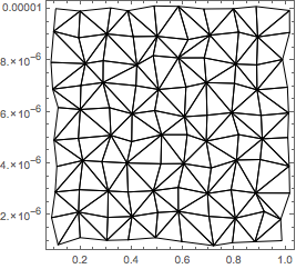
The interpolation is created with ElementMeshInterpolation as above:
if = ElementMeshInterpolation[{mesh}, values,
   "ExtrapolationHandler" -> {Indeterminate &, "WarningMessage" -> False}];
Plotting:
ContourPlot[if[x, y],
 Evaluate[Sequence @@ Transpose[Join[{{x, y}}, Transpose[if["Domain"]]]]]]
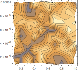
There are still some glitches near the border. These are probably from triangles having some vertices lying outside the domain of if. (I'm speaking of triangles created by ContourPlot in its recursive subdivision of the domain.) These might also be due to ContourPlot trying to find the edge of the domain or from a problem with RegionMember. The option RegionFunction -> (if[#1, #2] =!= Indeterminate &) cleans up the edges, but the option setting RegionFunction -> RegionMember[MeshRegion[if["ElementMesh"]]] produces the graph above.
Quicker but more ragged plotting
Given the approximate nature of a linear interpolation, perhaps a fairly accurate and speedy method of plotting is good enough. It certainly could be good enough for "rough draft" purposes. If the grid points are not far off center, they can be fed to ContourPlot to ensure the main features will be present. Doing so effectively stops the recursive subdivision, which where we save time. The initial sample point grid of ContourPlot should be constructed so that the points in our data grid land in the middle of the sample point grid. There are two answers to Specific initial sample points for 3D plots that give an extensive analysis of this method of specifying PlotPoint. Please consult them for further explanation.
Pass a mesh interpolation if and the dimensions of the grid to ifContourPlot. It figures out the mean grid spacing and adds a half grid to all sides of the plot domain. If PlotPoints are specified to be dim + 1, then the grid points will be approximately in the center of each plot-point grid cell.
Clear[ifContourPlot];
ifContourPlot[if_, dim_, opts___] := Module[{domain, dx, dy},
  domain = if["Domain"];
  {dx, dy} = Flatten[Differences /@ domain]/dim/2;
  With[{plotdomain =
     Transpose[Join[{{x, y}}, Transpose[{{-dx, dx}, {-dy, dy}} + domain]]]},
   ContourPlot[if[x, y], Evaluate[Sequence @@ plotdomain],
    Epilog -> {Red, Point["grid" /. opts /. "grid" -> {}]},
    PlotRange -> if["Domain"], PlotRangePadding -> Scaled[0.01],
    Evaluate@FilterRules[{opts}, Options[ContourPlot]]]
   ]];
We add the mesh coordinates, which are the same as grid, to the automatic plot points. This takes 0.06 sec. compare to 1 sec for the regular ContourPlot above.
ifContourPlot[if, {10, 10},
 PlotPoints -> {10 + 1, if["ElementMesh"]["Coordinates"]}]
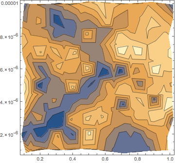
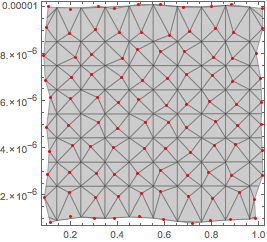
Here are the sample points and the mesh generated by ContourPlot. The contours are line segments connecting edges of the mesh (determined, I would guess, by linear interpolation between the sample points).
ifContourPlot[if, {10, 10},
 PlotPoints -> {10 + 1, if["ElementMesh"]["Coordinates"]},
 Mesh -> All, Contours -> 0,
 Epilog -> {Red, Point[if["ElementMesh"]["Coordinates"]]}]


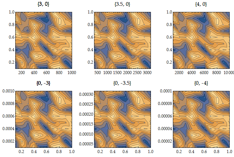
Method -> {"DelaunayDomainScaling" -> True}in the contour plot to work around this issue. Unfortunately it doesn't seem to work in version 10. $\endgroup$DataRangeMMA want's to be smart and rescale sampling :/. Is my workarund ok? $\endgroup$