18
$\begingroup$

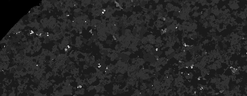
I am trying to quantify the proportions of various components in a greyscale image (backscattered electron image of a polished rock sample). Here is the original image:

bse = Import@"https://i.sstatic.net/eQece.png";
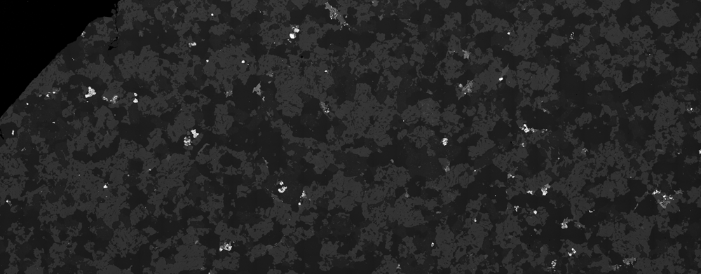
enter image description here

The image is comprised of components (minerals) that should have the same intensity response. For example, the abundant 'mid-grey' component (plagioclase) should have a fixed grey-level across the entire image. It doesn't.

By masking the other components of the image and adjusting the contrast, the gradations in brightness become more obvious:

bsek = ImageSubtract[bse, ColorNegate@Binarize[bse, {0.16, 0.24}]];
ImageAdjust[bsek, {3, 1.1}]
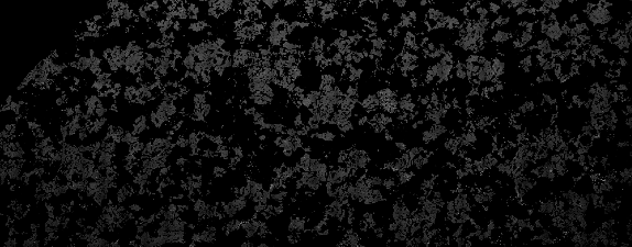
enter image description here

There seems to be two effects: a first order decrease in brightness towards the bottom corners and a second-order periodic vertical striping (comprised of short wavelength gradients).

Why bother? - Correcting for variations in brightness is an important step prior to segmentation analysis of the image

By approximating the variation in grey-values for the plagioclase, the difference in birghtness between the top and bottom of the image can be modelled (albeit crudely).

ksim[im_] := Module[{kdf, kdl},
  kdf = SmoothKernelDistribution[First@im];
  kdl = SmoothKernelDistribution[Last@im];
  Plot[{PDF[kdf, x], PDF[kdl, x]}, {x, 0, 0.3}, Filling -> Axis, 
   Exclusions -> None]]
ksim[ImageData[bsek]]
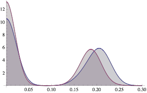
enter image description here

The following creates a gradational filter that causes the grey-level peaks to overlap (by adjusting the value of shift).

bsedim = ImageDimensions[bse]
shift = 0.2;
grad = 1 + 
   Transpose@
    Array[Table[x, {x, -shift, 0., shift/bsedim[[1]]}] &, bsedim[[1]]];
gradi = Image[grad];

bsekm = ImageMultiply[bsek, gradi];
ksim[ImageData[bsekm]]
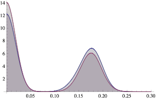
enter image description here

This filter can then be applied to the original image:

bsem = ImageMultiply[bse, gradi]
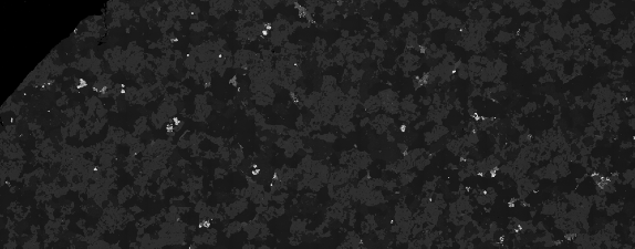
enter image description here

This clumsy method does an OK job of levelling the first-order brightness defect. However, this effect looks to have a spherical gradient (dimmer in the bottom corners than the middle) which is not accounted for.

As yet, I have not found a way to correct the second order periodic effect.

Can anyone suggest a more straightforward way to detect and correct these kinds of brightness variation defects? Extra bonus gratitude to anyone who can help to correct the second-order periodic aberration.


Update

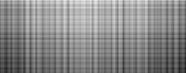
Here is a contrast stretched image showing the vertical aberrations:

 ImageAdjust[bse, {4.5, 3.85}]
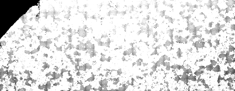
enter image description here

$\endgroup$
0

3 Answers 3

12
$\begingroup$

Does this help? I've treated the error as additive, though you could easily change it to a multiplicative correction.

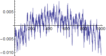
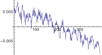
Starting with your bsek image, find the mean offset for rows and for columns:

id = ImageData[bsek];
horiz = (# - Mean[#]) &[Total[id]/Total[Unitize[id]]];
vert = (# - Mean[#]) &[Total[id, {2}]/Total[Unitize[id], {2}]];

ListLinePlot[horiz]
ListLinePlot[vert]

enter image description here enter image description here

The horizontal plot shows an overall darkening at the left and right sides of the image, plus the periodic component. The vertical plot shows an overall darkening towards the bottom of the image, with a periodic component also.

Combining the horizontal and vertical offsets into an overall offset:

a = Outer[Plus, vert, horiz];
Image[a] // ImageAdjust

enter image description here

Now subtract the offset from the original data:

bse2 = Image[ImageData[bse] - a]

enter image description here

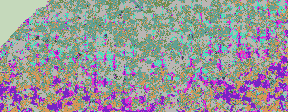
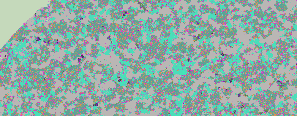
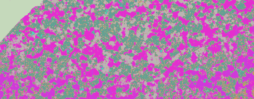
Using s.s.o.'s ClusteringComponents visualisation appears to show an improvement:

ClusteringComponents[bse, 10] // Colorize
ClusteringComponents[bse2, 10] // Colorize

enter image description here enter image description here

$\endgroup$
5
  • $\begingroup$ This is a really great approach! Many Thanks! There seems to be a 'noise' issue with respect to the vertical and horizontal lines. This is visible if you adjust the contrast, e.g. ImageAdjust[bse2, {4.5, 3.85}]. Perhaps there is some way of smoothing the curves?.. $\endgroup$
    – geordie
    Commented Aug 21, 2013 at 12:01
  • 2
    $\begingroup$ I think the problem is that a correction determined at one brightness level does not necessarily apply at another. Ideally you would determine the detector response at multiple signal levels and apply a compensation curve rather than the single-point correction I have shown. Even then, you will still have residual error because of quantisation noise. Of course, there is also an assumption in my approach that the detector non-uniformity is separable into horizontal and vertical components, which won't in general be true. $\endgroup$ Commented Aug 21, 2013 at 13:50
  • $\begingroup$ @SimonWoods,I have a Question. Not that I know very well. If I look dat = ImageData@bse2; dat1 = ImageData@img; EuclideanDistance[dat, dat1] I get 2.50524 and only dat2 = ColorQuantize[img, 10, Dithering -> False]; EuclideanDistance[dat, ImageData@dat2] I get 2.35325. So, If the value is bigger does that mean you lose more information? Or how can we measure any ideas. Just out of my curiosity. $\endgroup$
    – s.s.o
    Commented Aug 21, 2013 at 14:23
  • $\begingroup$ @s.s.o, I'm not sure what you mean. Surely EuclideanDistance is just measuring how different the images are? $\endgroup$ Commented Aug 21, 2013 at 15:14
  • $\begingroup$ Simon, you know a lot more about this stuff than I. For my purposes your solution works well. I reprocessed the image using a mask generated from the darkest mineral (quartz). The v and h curves are a lot smoother and the correction seems to work better. Thanks again! $\endgroup$
    – geordie
    Commented Aug 21, 2013 at 23:49
2
$\begingroup$

I now know it is now what OP is looking for exactly, but till there is no better approach I will leave this answer.

dat = ImageData @ pic;
Histogram[dat // Flatten]

enter image description here

Image@Round[dat, .05]

enter image description here

$\endgroup$
7
  • $\begingroup$ Unfortunately not. I am trying to avoid losing 'fidelity' in the grey-levels. There are some very dark components that have very close grey-level ranges. You can see them in my raw and filtered images but they are lost from your filtered image. Thanks for trying. $\endgroup$
    – geordie
    Commented Aug 21, 2013 at 6:04
  • $\begingroup$ This is better for sure, but it is still downsampling the grey-levels(which i would prefer not to do). It might be good enough. I will test it one some other images and let you know. $\endgroup$
    – geordie
    Commented Aug 21, 2013 at 6:42
  • 1
    $\begingroup$ @geordie I do not expect it to be a the general approach, I wanted to try if this simple approach can be useful for you. About aberrations, are they on each image? Can you make a plain image with only those variations? If yes, normalize it and divide your measurement images by this so-called "flat". $\endgroup$
    – Kuba
    Commented Aug 21, 2013 at 6:45
  • $\begingroup$ Alas, I cannot obtain a plain image. That would be a great solution as it would probably remove both effects at once. $\endgroup$
    – geordie
    Commented Aug 21, 2013 at 6:59
  • $\begingroup$ I had a good look at the filtered image and, unfortunately, too much information is lost (even with the 0.5 rounding). $\endgroup$
    – geordie
    Commented Aug 21, 2013 at 7:09
1
$\begingroup$

Is this sort of what you need as a result? It's simple approach but I'll delete if it's not you asked for.

img = Import@"https://i.sstatic.net/eQece.png";

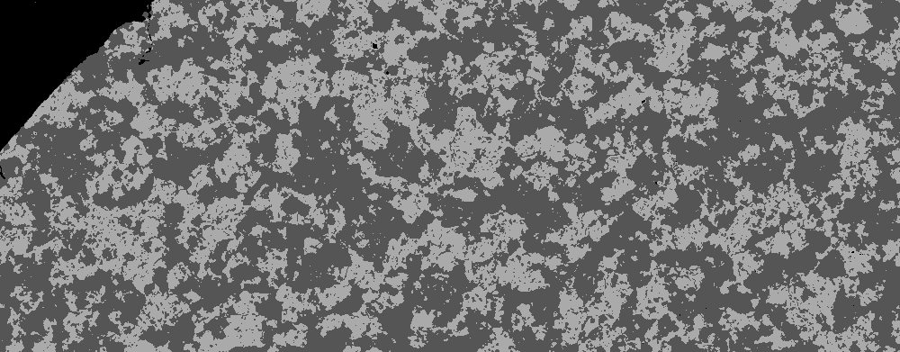
cl = ClusteringComponents[img];
im = Colorize[cl, ColorFunction -> GrayLevel]

you get

enter image description here

Edit 1

if you know roughly component numbers you can use

cl = ClusteringComponents[img, 10];
im = Colorize[cl]

enter image description here

Edit 2

Based on the solution by cormullion in his answer. (Sightly modified) You can quantify colors.

colorquantized = SortBy[Tally[Flatten[
 ImageData[ColorQuantize[img, 12, 
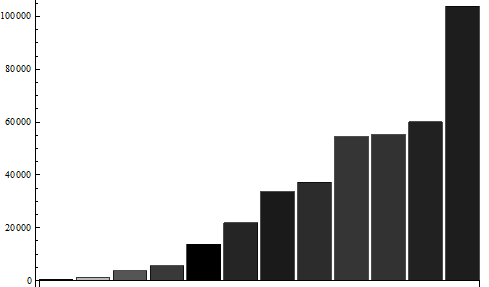
   Dithering -> False]], 1]], Last]

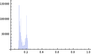
{{0.0823529, 482}, {0.72549, 1306}, {0.333333, 3627}, {0.223529, 5561}, {0., 13718}, {0.145098, 21902}, {0.101961, 33696}, {0.172549, 37135}, {0.207843, 54467}, {0.196078, 55245}, {0.129412, 60045}, {0.113725, 103816}}

BarChart[colorquantized[[All, 2]], 
 ChartStyle -> GrayLevel /@ colorquantized[[All, 1]]]

enter image description here

Than you can use clustering to find colors to group to best fit to your purpose by:

FindClusters[colorquantized[[All, 2]], 7]

{{482, 1306}, {3627}, {5561}, {13718}, {21902}, {33696, 37135}, {54467, 55245, 60045, 103816}}

and if you like the number of clusters are ok. you use it

cl = ClusteringComponents[img,7];
im = Colorize[cl]

enter image description here

One disadvantage of this approach is choosing the number of clusters in a nice way (analytic way).

$\endgroup$
5
  • $\begingroup$ No, this approach results in a huge loss in 'fidelity'. The grey-levels are reduced to three levels. All the data for the other components are lost. Thanks anyway. $\endgroup$
    – geordie
    Commented Aug 21, 2013 at 9:26
  • $\begingroup$ Ok. By the way you can adjust the component numbers and get those... You can also try MeanShiftFilter... $\endgroup$
    – s.s.o
    Commented Aug 21, 2013 at 9:35
  • $\begingroup$ you may also interested in this answer about dominant colors as an alternative. mathematica.stackexchange.com/questions/24898/… $\endgroup$
    – s.s.o
    Commented Aug 21, 2013 at 9:41
  • $\begingroup$ Thanks for the suggestions. I have played around with MMA's morphological tools and filters. I will try to use these once the image is 'balanced'. As your second image clearly shows there are first and second order aberrations that interfere with the textural information in the image (the minerals). Removing these aberrations is a necessary first step before applying segmentation tools. $\endgroup$
    – geordie
    Commented Aug 21, 2013 at 10:10
  • $\begingroup$ Yes. The question is now clearer. Good luck with it. $\endgroup$
    – s.s.o
    Commented Aug 21, 2013 at 10:17

Your Answer

By clicking “Post Your Answer”, you agree to our terms of service and acknowledge you have read our privacy policy.

Not the answer you're looking for? Browse other questions tagged or ask your own question.