The below code executes. If I uncomment the Plot, it runs for a while and outputs nothing, not even the Mean and Variance.
new2 = TransformedDistribution[(x + y + z)/3, {x, y,z} \[Distributed] LogMultinormalDistribution[{0,1,0},{{1,0,0},{0,1,0},{0,0,1}}]];

lmdpdf = PDF[new2,x];

(* Plot[%, {x, 1, 8}, Filling -> Axis,PlotRange -> Automatic]  *)

Mean[new2]
Variance[new2]
========
Meanwhile, the below works fine.
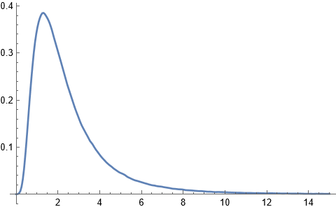
new2a = TransformedDistribution[(x + y),
 {x\[Distributed] NormalDistribution[],
y \[Distributed] NormalDistribution[]}
];

PDF[new2a, x];

Plot[%, {x, -6, 8}, Filling -> Axis,PlotRange -> Automatic]

Mean[new2a]
Variance[new2a]
===
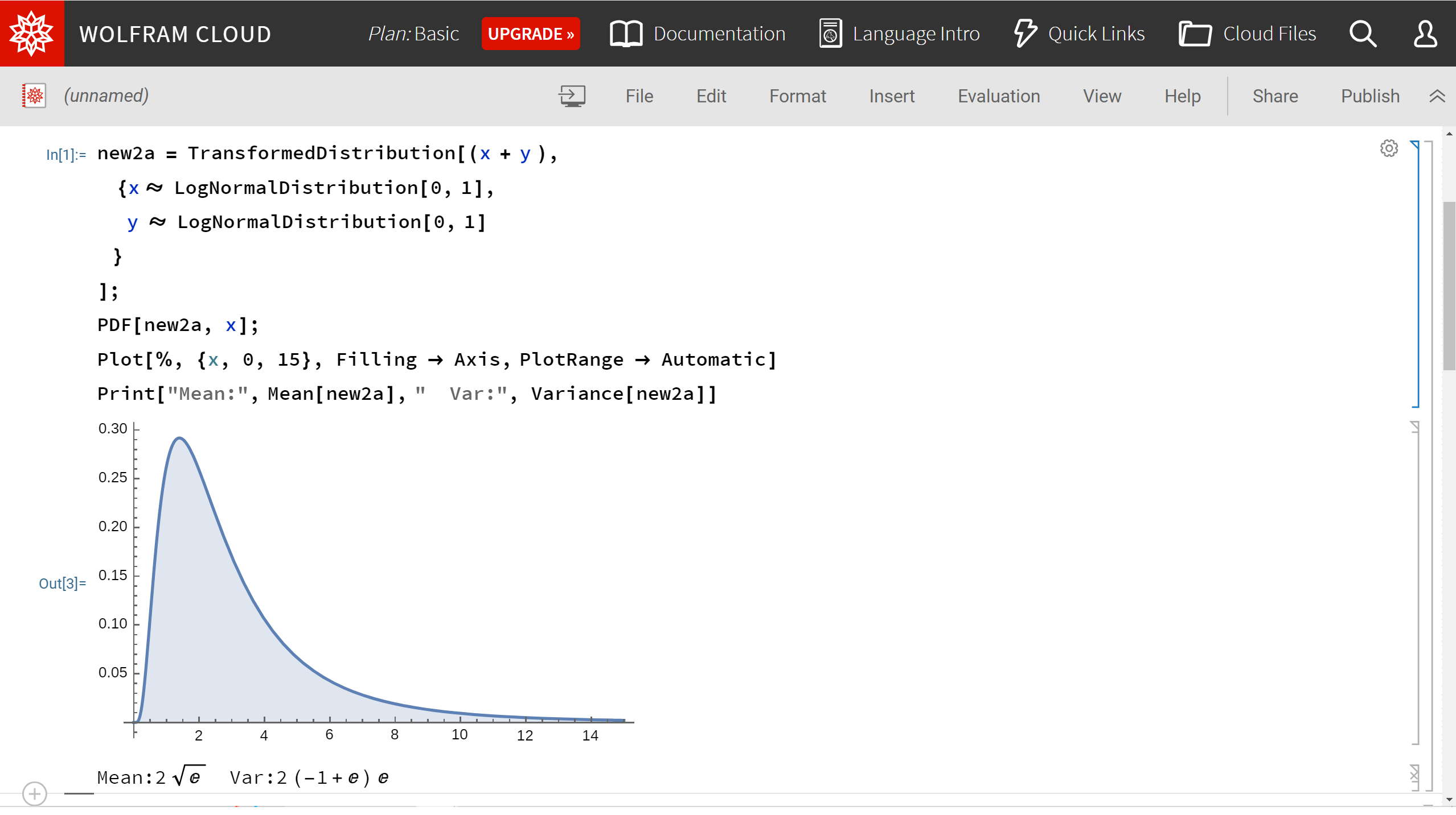
ADDED in response to comment. The below runs fine, including plot. I think it is the same as a 2 variable version of my non-plotting Transform.
===
new2a = TransformedDistribution[(x + y),
 {x\[Distributed] LogNormalDistribution[0,1],
y \[Distributed] LogNormalDistribution[0,1]
}
]
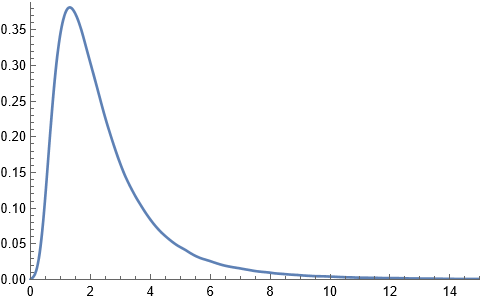
Added more: tried exactly two variable version, and it fails to plot. Sans Plot function, it returns the same Mean and Variance though, so I am even more confused. This is apparently not a Plot issue, but a closed/open form issue combined with a built-in-symbols question...
new2 = TransformedDistribution[(x + y + z), {x,y,z} \[Distributed] LogMultinormalDistribution[{0,1,0},{{1,0,0},{0,1,0},{0,0,1}}]];
dividing by 2 (see below) also causes code to fail, which doesn't feel like it is a closed/open form issue, but I have no idea what MMA is doing under the covers ...
new2a = TransformedDistribution[(x + y)/2,
 {x\[Distributed] LogNormalDistribution[0,1],
y \[Distributed] LogNormalDistribution[0,1]
}
]


new2) is a univariate distribution. $\endgroup$PDF[new2a, 3.5]) allows Mathematica to produce a density.PDF[new2a, 7/2]doesn't return a density. So maybe there's an underlyingNPDFfunction (similar toNIntegrate). More to think about. $\endgroup$PDFand Mathematica recognizes that the distribution is the sum of two independent random variables, numerical convolution is used. See en.wikipedia.org/wiki/Convolution_of_probability_distributions. But it doesn't do this for a sum of 3 or more independent random variables.PlotfeedsPDFwith machine precision numbers so it works. And there still isn't a closed-form solution. $\endgroup$PDF(which I should have done earlier) under "Possible Issues" shows an example where the closed-form does not exist (and not for a sum of 2 independent random variables) but evaluates the pdf numerically. So there are multiple circumstances wherePDFcan kick into numerical mode. $\endgroup$