I would like to plot these following parametrizations:
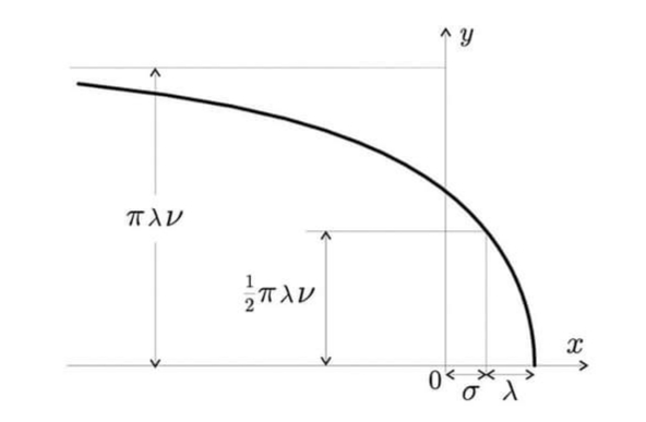
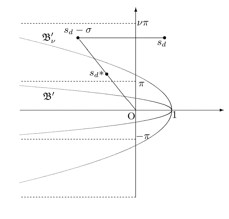
$$s(\theta)=\sigma+\lambda s_{\nu}(\theta),\quad s_{\nu}(\theta)=\theta\cot(\theta) + i\nu\theta,\quad \theta\in(-\pi,\pi)$$
For more details, please see: The accurate numerical inversion of Laplace Transform by A. Talbot.
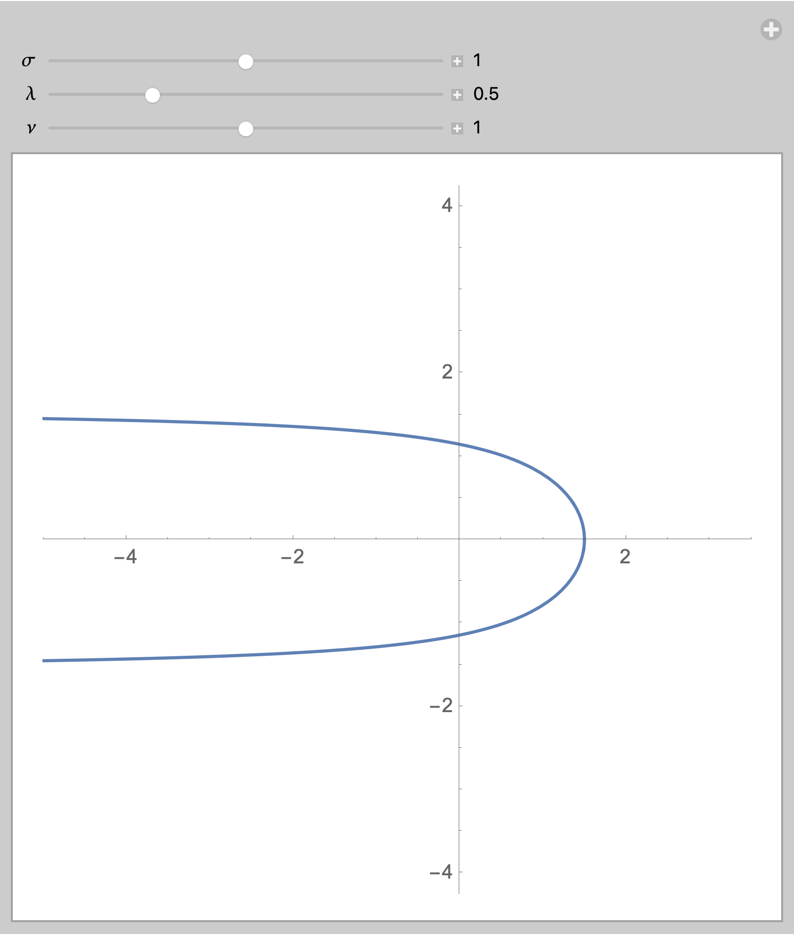
The parameters $\sigma$, $\lambda$, and $\nu$ are adjustable.
The Talbot's contour should looks like these two:
 Or
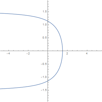
Or

My attempt:
σ := 1
λ := 1/2
ν := 1
s1 := θ*Cot (θ) + (I ν θ)
eqn := σ + (λ s1), Assumptions -> -Pi <= θ <= Pi
ParametricPlot[{Re[eqn], Im[eqn]}, {f, -5, 2}, AspectRatio -> 1]
Sorry, I can't give further attempt since I'm not really familiar with Mathematica. Hope you can help me. Thanks in advance.


:=) for assignments to constants. 2)Assumptionsis an option of only certain functions. You can't use it that way. Didn't you see the error when you tried to execute your code? 3) Functions in MMA enclose their parameters in[], soCot[theta]and notCot(theta). 4) The variable in ParametricPlot should be the same as in your equation, i.e. theta, notf. $\endgroup$