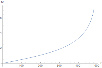
I try to evaluate this symbolic integral and evaluate its two series expansions according to certain variables, the plot the output providing some numerical values.
This is a relativistic rotational hollow disk. This one my thought experiments I try to figure it out. I am a hobbyist physicist
f1 = (y (-z +
       y Cos[x]))/(((1 - (\[Omega] y)^2/h^2)^(1/2)) ((z^2 + y^2 -
         2 z y Cos[x])^(3/2)));
f2 = Assuming[0 < z < 0.99 ymin  && 0.99 h > \[Omega] y,
   Integrate[f1, {y, ymin, ymax}, {x, 0, 2 Pi}] // FullSimplify];
S2 = Assuming[0 < z < 0.99 ymin  && 0.99 h > \[Omega] y,
  Series[f2, {z, 0, 3}, {\[Omega], 0, 4}] // FullSimplify]
S3 = Assuming[0 < z < 0.99 ymin  && 0.99 h > \[Omega] y,
  Series[f2, {w, 0, 3}] // FullSimplify]
\[Omega] = 1;
w = z \[Omega]^2;
h = 1000;
ymin = 500;
ymax = 985;
Plot[f2, {w, 0, 495}]
My Question is: I takes very very long time, and I lost the hope to see result. I use the trial version of the most recent Mathematica.
Is there something wrong in this code?
------------ at Aug 28 2020 --------------
What if I try to fix z and plot versus omega provided that ymin>z>ymax. There will be divergence at z, so I tried to divide the integral to two integrals and take the limit at z to solve the improper integrations, the one that has ymin1>z>ymax1, and the other that has ymin2>z>ymax2. It didn't give me any result. Here is a trial to fix z and do series and plot with respect to omega.
f1[z_?NumericQ, \[Omega]_?NumericQ, h_?NumericQ, ymin1_?NumericQ,
   ymax1_?NumericQ] :=
  NIntegrate[(y (-z +
        y Cos[x]))/(((1 - (\[Omega] y)^2/h^2)^(1/2)) ((z^2 + y^2 -
          2 z y Cos[x])^(3/2))), {y, ymin1, ymax1}, {x, 0, 2 Pi},
   Method -> "LocalAdaptive"];
f2[z_?NumericQ, \[Omega]_?NumericQ, h_?NumericQ, ymin2_?NumericQ,
   ymax2_?NumericQ] :=
  NIntegrate[(y (-z +
        y Cos[x]))/(((1 - (\[Omega] y)^2/h^2)^(1/2)) ((z^2 + y^2 -
          2 z y Cos[x])^(3/2))), {y, ymin2, ymax2}, {x, 0, 2 Pi},
   Method -> "LocalAdaptive"];
f3 = f1 + f2;
L1 = Limit[f1[1, \[Omega], 1000, 0, ymx1], ymx1 -> 1,
  Assumptions -> ymx1 < 1]
L2 = Limit[
  f2[1, \[Omega], 1000, ymn2, ymx2], {ymn2 -> 1, ymx2 -> 250},
  Assumptions -> ymn2 > 1 && ymx2 < 250  && \[Omega] < 4]
L3 = L1 + L2

S1 = Series[L1, {\[Omega], 0, 4}]
S2 = Series[L2, {\[Omega], 0, 4}]
S3 = Series[(L1 + L2), {\[Omega], 0, 4}]

P1 = Plot[L1, {\[Omega], 0, 4}, AxesLabel -> {"\[Omega]", "L1"}]
P2 = Plot[L2, {\[Omega], 0, 4}, AxesLabel -> {"\[Omega]", "L2"}]
P3 = Plot[(L1 + L2), {\[Omega], 0, 4},
  AxesLabel -> {"\[Omega]", "L3"}]
And what if I need to get series and plot w.r.t. z also?


w = z \[Omega]^2andf2will have a mixture ofyandz. Plot needs a single independent variable. $\endgroup$